5
Chapter 3
Recent Change in the Arctic and the Arctic Oscillation
¡¡¡¡¡¡¡¡¡¡¡¡¡¡¡¡¡¡¡¡¡¡¡¡¡¡¡¡¡¡¡¡¡¡¡¡¡¡¡¡¡¡¡¡¡¡¡¡¡¡¡¡¡¡¡¡¡¡¡¡¡¡¡¡¡¡¡¡¡¡¡¡¡¡¡¡¡¡¡¡¡¡¡¡¡¡¡¡¡
Because the AO is usually `smoothed', it does not ade-
3.1. The Arctic Oscillation
quately represent events and short-term variations
During the 1990s, a quiet revolution took place in the
which are known to be important for the delivery of
perception of the Arctic (Carmack et al., 1997; Dickson,
contaminants to the Arctic and possibly also locally im-
1999; Johannessen et al., 1995; Johnson and Polyakov,
portant in forcing ice and surface water motion (see for
2001; Kerr, 1999; Levi, 2000; Macdonald, 1996; Mac-
example, Sherrell et al., 2000; Welch et al., 1991). It is
donald et al., 1999a; Maslanik et al., 1996; Maslowski
important to note that one of the projections of climate
et al., 2000; McPhee et al., 1998; Morison et al., 1998,
change is that cyclonic activity will increase; extreme
2000; Parkinson et al., 1999; Polyakov and Johnson,
events may therefore become a prominent component of
2000; Quadfasel et al., 1991; Smith, 1998; Steele and
atmospheric transport in the coming century. The earli-
Boyd, 1998; Vanegas and Mysak, 2000; V÷r÷smarty et
est significant rain event on record (May 26, 1994),
al., 2001; Walsh, 1991; Welch, 1998; Weller and Lange,
which was observed widely throughout the Canadian
1999). Despite early evidence of cyclical change in north-
Arctic Archipelago may have represented an example of
ern biological populations and ice conditions (e.g., Bock-
this (see also Graham and Diaz, 2001; Lambert, 1995).
stoce, 1986; Gudkovich, 1961; Vibe, 1967), the general
Around 1988 to 1989, the AO entered a positive
view among many western physical scientists through-
phase of unprecedented strength (Figures 3À1 a and c,
out the 1960s to 1980s was that the Arctic was a rela-
next page). The sea-level pressure (SLP) distribution pat-
tively stable place (Macdonald, 1996). This view has
tern of the AO for winter and summer (Figures 3À1 b and
been replaced by one of an Arctic where major shifts can
d) shows that this positive shift in AO is characterized
occur in a very short time, forced primarily by natural
by lower than average SLP distributed somewhat sym-
variation in the atmospheric pressure field associated
metrically over the pole (the blue-isoline region on Fig-
with the Northern-hemisphere Annual Mode.
ures 3À1 b and d) and higher SLP over the North Atlantic
The Northern-hemisphere Annual Mode, popularly
and North Pacific in winter and over Siberia and Europe
referred to as the Arctic Oscillation (AO) (Wallace and
in summer. As might be expected from examination of
Thompson, 2002), is a robust pattern in the surface man-
the AO SLP pattern (Figures 3À1 b and d), when the AO
ifestation of the strength of the polar vortex (for a very
index is strongly positive conditions become more `cy-
readable description, see Hodges, 2000). The AO corre-
clonic' ¡ i.e., atmospheric circulation becomes more
lates strongly (85-95%) with the more commonly used
strongly counterclockwise (Proshutinsky and Johnson,
indicator of large-scale wind forcing, the North Atlantic
1997; Serreze et al., 2000).
Oscillation (NAO) (the NAO is the normalized gradient
In discussing change it is important to distinguish be-
in sea-level air pressure between Iceland and the Azores
tween variability, which can occur at a variety of time
¡ see for example, Deser, 2000; Dickson et al., 2000;
scales (Fischer et al., 1998; Polyakov and Johnson,
Hurrell, 1995; Serreze et al., 2000). In this report the
2000) and trends caused, for example, by GHG warm-
AO and NAO are used more or less interchangeably be-
ing. It has been suggested that locking the AO into a
cause they carry much the same information. It is recog-
positive mode might actually be one way that a trend
nized, however, that in both cases the term `oscillation'
forced by GHGs can manifest itself in the Arctic (Shin-
is rather misleading because neither index exhibits quasi-
dell et al., 1999). Others, however, consider that the ex-
periodic behaviour (Wallace and Thompson, 2002). The
traordinary conditions of the 1990s were produced nat-
AO captures more of the hemispheric variability than
urally by a reinforcing of short (5-7 yr) and long (50-80
does the NAO which is important because many of the
yr) time-scale components of SLP variation (Polyakov
recent changes associated with the AO have occurred in
and Johnson, 2000; Wang and Ikeda, 2001), and that
the Laptev, East Siberian, Chukchi and Beaufort Seas ¡ a
GHG forcing will affect the mean property fields rather
long way from the NAO's center of action (Thompson
than alter the AO itself (Fyfe, 2003; Fyfe et al., 1999).
and Wallace, 1998). Furthermore, the Bering Sea and the
Longer records of the NAO index (Figure 3À16 a, page
Mackenzie Basin are both influenced to some degree by
18) indeed suggest that there have been other periods of
atmospheric processes in the North Pacific (e.g., the Pa-
high AO index during the past 150 years (e.g., 1900-
cific Decadal Oscillation; see also Bjornsson et al., 1995;
1914), but none as strong as that experienced during the
Niebauer and Day, 1989; Stabeno and Overland, 2001),
early 1990s. Recent data suggest that the AO index has
whereas the Baffin Bay ice climate appears to have an as-
decreased and that the Arctic system has to some degree
sociation with the Southern Oscillation (Newell, 1996),
begun to return to `normal conditions' (Bj÷rk et al.,
and the Canadian Arctic Archipelago and Hudson Bay
2002; Boyd et al., 2002; Johnson et al., 1999).
probably respond to various atmospheric forcings as yet
The contrast in conditions between the Arctic in the
not fully understood.
1960s, 1970s and 1980s (with a generally low/negative
Although the AO is an important component of
AO index) and the Arctic in the early 1990s (with an ex-
change in Arctic climate, it accounts for only 20% of the
ceptionally high/positive AO index) provides an extraor-
variance in the atmospheric pressure field and many
dinary opportunity to investigate how the Arctic might
other factors can determine the atmospheric forcing.
respond to climate change. Similarity between climate-
6
AMAP Assessment 2002: The Influence of Global Change on Contaminant Pathways
Winter Arctic Oscillation index
Summer Arctic Oscillation index
+1
+1
a
c
0
0
¡1
¡1
1960
1970
1980
1990
2000
1960
1970
1980
1990
2000
Winter Arctic Oscillation pattern
Summer Arctic Oscillation pattern
b
d
0
0
¡2
¡1
1
¡4
¡2
0
1
2
Figure 3À1. The Arctic Oscillation. The figure illustrates a) variability in the AO index between 1958 and 1998 in winter; b) the associated
winter sea-level pressure pattern; c) variability in the AO index between 1958 and 1998 in summer; and d) the associated summer sea-level
pressure pattern. To recreate atmospheric pressure patterns during the period in question, the winter (b) and summer (d) AO patterns would
be multiplied by their respective indices (a, c) and added to the mean pressure field. Thus the high winter AO index in the early 1990s implies
anomalously low pressure over the pole in the pattern shown in (b). Small arrows show the geostrophic wind field associated with the AO
pattern with longer arrows implying stronger winds.
change projections and AO-induced change suggests
the Atlantic Ocean through the deep connection at Fram
that examining the differences between AO¡ and AO+
Strait. Ocean circulation within the Arctic is tightly tied
states should provide insight into the likely effects of cli-
to bathymetry through topographic steering of currents
mate change forced by GHG emissions. Variation in
(Rudels et al., 1994). Considering these kinds of con-
SLP, as reflected by the AO index, demonstrates that the
straints, rapid change can occur in ocean-current path-
Arctic exhibits at least two modes of behaviour (Mori-
ways or in the source or properties of the water carried
son et al., 2000; Proshutinsky and Johnson, 1997) and
by currents when, for example, fronts shift from one ba-
that these modes cascade from SLP into wind fields, ice
thymetric feature to another (McLaughlin et al., 1996;
drift patterns, watermass distributions, ice cover and
Morison et al., 2000), when a given current strengthens
probably many other environmental parameters.
or weakens (Dickson et al., 2000), when source-water
The Arctic is to a large degree constrained by overar-
composition alters (Smith et al., 1998; Swift et al.,
ching structures and processes in how it can respond to
1997), or when relative strength of outflow varies be-
change. As illustrated in previous assessments, the Arctic
tween the Canadian Arctic Archipelago and Fram Strait
Ocean is, and will remain, a `mediterranean' sea, much
(Macdonald, 1996), but not by reversal of flow in
influenced by land¡ocean interaction and with restricted
boundary currents or reversal of mean flow in the Bering
exchange with other oceans (Figure 1À1). Topography,
Strait or out through the Archipelago.
bathymetry and global distribution of salinity in the
Change associated with the Northern-hemisphere
ocean, require that water from the Pacific Ocean will
Annual Mode requires that consideration be given to
predominantly flow in to the Arctic and the shallow sill
large-scale variability in the Arctic; the fact that physical
at Bering Strait (50 m) guarantees that only surface
pathways can change rapidly needs to be recognized in
water will be involved in this exchange. Pacific water
greater detail, and the potential effects of GHG emis-
will remain above Atlantic Layer water which is denser.
sions against this naturally variable background should
Deep-basin water communicates predominantly with
be assessed.
Recent Change in the Arctic and the Arctic Oscillation
7
Positive Arctic Oscillation Index (AO+)
Negative Arctic Oscillation Index (AO ¡)
(cyclonic)
(anticyclonic)
Aleutian Low
Winter
1015
a
1015
b
L
L
1015
1015
1015
1025
H
H
L
L
1005
1015
H
Icelandic Low
Siberian High
Positive Arctic Oscillation Index (AO+)
Negative Arctic Oscillation Index (AO ¡)
(cyclonic)
(anticyclonic)
Beaufort High
H
Summer
H
c
d
1018
1018
1014
1014
1010
1010
1014
1014
L
L
L
1010
1018
1014
1018
1006
H
H
Figure 3À2. Atmospheric pressure fields and wind stream lines in the Northern Hemisphere. The figure illustrates a) strong AO+ conditions in
winter; b) strong AO¡ conditions in winter; c) strong AO+ conditions in summer; and d) strong AO¡ conditions in summer.
2001; Proshutinsky and Johnson, 1997) thereby indi-
3.2. Winds
rectly affecting transport by these two media as well.
Winds transport contaminants directly to the Arctic by
To understand how swings in the AO can affect at-
delivering volatile and semi-volatile chemicals, and chem-
mospheric circulation, AO+ and AO¡ wind field/SLP
icals attached to fine particulates, from the south in
maps have been constructed for winter (Figures 3À2 a
timescales as short as a few days (Bailey et al., 2000;
and b) and summer (Figures 3À2 c and d) by adding
Barrie et al., 1998; Halsall et al., 1998; Hung et al.,
(AO+) or subtracting (AO¡) the patterns in Figures 3À1 b
2001; Stern et al., 1997). Over the longer term, spanning
and d to/from the mean pattern for the period of record
months to years, winds deliver volatile and semi-volatile
in the time series (1958-1998). The changes discussed in
contaminants through a series of hops, as airborne
the following paragraphs can be considered generally as
chemicals become deposited onto surfaces (water, soil or
representing the difference between conditions during
vegetation) and then re-volatilized during, for example,
the 1960s to 1970s (low/negative AO index) and during
summer warming. Winds also provide the primary forc-
the early 1990s (high/positive AO index) (see for exam-
ing for ice drift and surface ocean currents (Mysak,
ple, Proshutinsky and Johnson, 1997).
8
AMAP Assessment 2002: The Influence of Global Change on Contaminant Pathways
In winter (Figures 3À2 a and b), the lower tropos-
cording to Iversen (1996) summer accounts for only
pheric circulation is dominated by high pressure over the
20% of the annual south-to-north air transport (souther-
continents and low pressure over the northern Pacific
lies in the Norwegian Sea (10%), Eastern Europe/Siberia
Ocean (Aleutian Low) and Atlantic Ocean (Icelandic
(5%), and Bering Sea (5%)). The streamlines show that
Low). The Siberian High tends to force air on its western
winds provide a means to transport contaminants from
side into the Arctic, acting as an effective atmospheric
industrialized North America and Europe to the North
conduit from industrialized regions of Siberia and East-
Atlantic but penetration into the Arctic weakens. In the
ern Europe to the High Arctic. The high-pressure ridge
North Pacific, there remain atmospheric pathways to
over North America then forces air southward giving a
move air masses into the Gulf of Alaska from the east
net transport out of Eurasia into the Arctic, across the
coast of Asia (Figures 3À2 c and d). During AO+ condi-
Arctic and south over North America. The Icelandic
tions in particular, the Beaufort High weakens or disap-
Low produces westerly winds over the eastern North At-
pears (Figures 3À2 a and c), altering mean wind fields.
lantic and southerly winds over the Norwegian Sea pro-
viding a second conduit by which airborne contaminants
3.3. Surface air temperature
from eastern North America and Europe can rapidly
reach the Arctic. Finally, the Aleutian Low tends to steer
A strong trend of warming has been observed in the Arc-
air that has crossed the Pacific from Asia up into Alaska,
tic for the period from 1961 to 1990 (Figure 3À3 a). This
the Yukon, and the Bering Sea (Bailey et al., 2000; Li et
warming, which has been especially evident over north-
al., 2002; Wilkening et al., 2000). During winter, these
western North America and Siberia, has been accompa-
three routes into the Arctic ¡ southerlies in the Norwe-
nied by cooling in northeastern Canada, Baffin Bay, and
gian Sea (40%), over Eastern Europe/Siberia (15%), and
West Greenland. An almost identical pattern of warming
over the Bering Sea (25%) account for about 80% of the
to that shown in Figure 3À3 a is produced by taking the
annual south-to-north air transport (Iversen, 1996).
difference between mean surface air temperatures during
With a higher AO index (Figure 3À2 a), the Icelandic
periods of AO+ and AO¡ conditions (Wallace and Thomp-
Low intensifies and extends farther into the Arctic
son, 2002). Due to an extensive temperature record col-
across the Barents Sea and into the Kara and Laptev Seas
lected from drifting buoys, manned drifting stations, and
(Johnson et al., 1999). This has the effect of increasing
land stations, direct relationships can be drawn between
the wind transport east across the North Atlantic, across
air surface temperature over sea and land in the Arctic
southern Europe and up into the Norwegian Sea. During
and the changes in pressure field discussed in section
high NAO winters, westerlies onto Europe may be as
3.2. Over the period 1979 to 1997, a trend of +1░C per
much as 8 m/s (~700 km/day) stronger (Hurrell, 1995).
decade was found for winter surface air temperature
At the same time, strong northerly winds are to be found
(SAT) in the eastern Arctic Ocean, offset by a trend of
over the Labrador Sea (Mysak, 2001).
¡1░C per decade in the western Arctic Ocean (Rigor et
The extension of the Icelandic Low into the Arctic
al., 2000). However, in spring almost the entire Arctic
also implies an effect of the AO on storm tracks. During
Ocean shows significant warming ¡ as much as 2░C per
the strong AO+ conditions of the early 1990s, there was a
decade in the eastern Arctic where a trend toward
remarkable increase in the incidence of deep storms, to
lengthened melt season was also observed. The trend in
around 15 per winter, and these storms penetrated farther
increasing SAT over the ocean is matched by tempera-
into the Arctic (Dickson et al., 2000; Maslanik et al., 1996;
ture increases over Arctic land masses of 2░C per decade
Semiletov et al., 2000). Increased cyclone activity increases
during winter and spring and annual increases of per-
poleward transport of heat and other properties carried by
haps 0.8░C per decade (Figure 3À3 a). Records of annual
the air masses involved. Anomalous southerly airflow over
temperature anomalies since 1900 (Figure 3À3 b) clearly
the Nordic Seas enhances the connection between indus-
show the warming trend since the 1970s, but note also
trial regions of North America and Europe and the Arctic.
that a similar episode of warming occurred in the 1930s
At the same time, increased cyclones enhance transfer of
to 1940s. Taken together, the trends in SAT over the cen-
contaminants from the atmosphere to the surface as a con-
tral Arctic Ocean suggest that warming has occurred
sequence of increased precipitation. Deep within the Arc-
predominantly during January to July (Figure 3À3 c).
tic, the high SLP ridge that extends across Canada Basin
Over half of the change in SAT in Alaska, Eurasia and
during AO¡ conditions (the Beaufort High), disappears
the eastern Arctic Ocean has been ascribed to the AO,
and withdraws toward Russia (Johnson et al., 1999;
but less than half in the western Arctic (see Dickson et
Morison et al., 2000). It is worth noting that the Pacific
al., 2000; Rigor et al., 2000; Serreze et al., 2000). The
mean atmospheric pressure field and wind patterns appear
temperature changes associated with the AO are consid-
to change little between strong positive and strong nega-
ered large enough to have an immediate effect on polar
tive phases of the AO in winter. Penetration of air from the
circulation (Morison et al., 2000).
Pacific into the Arctic is hindered by the mountain barrier
along the west coast of North America where intensive
3.4. Precipitation and runoff
precipitation also provides a mechanism to transfer con-
taminants and aerosols to the surface (Figures 3À2 a and b).
Precipitation is a key pathway for contaminant transport
Summer pressure fields and air-flow patterns are
(Figure 1À2); rain, snow and fog scavenge aerosols and
markedly different from those of winter (compare Fig-
gasses from the atmosphere to deposit them at the sur-
ures 3À2 a, b, c, and d). In summer, the continental high-
face (Chernyak et al., 1996; Li et al., 2002; Macdonald et
pressure cells disappear and the oceanic low-pressure
al., 2000a; Mackay and Wania, 1995; Malcolm and
cells weaken with the result that northward transport
Keeler, 2002; Wania and Mackay, 1999). Scavenging by
from low latitudes weakens (Figures 3À2 c and d). Ac-
precipitation may be relatively weak in the desert-like
Recent Change in the Arctic and the Arctic Oscillation
9
Temperature change,
Temperature anomaly, ░C
55-85░N
1961-1990
1.0
░C per decade
b
0.6 - 0.8
0.5
Average
0.5 - 0.6
0
1951-1980
0.4 - 0.5
¡ 0.5
¡ 1.0
0.2 - 0.4
North Pole
1900
1920
1940
1960
1980
0.1 - 0.2
Variation in surface air temperature, ░C
¡ 0.1 - 0.1
0.6
c
Central Arctic Ocean
¡ 0.2 - ¡ 0.1
0.4
¡ 0.3 - ¡ 0.2
0.2
¡ 0.4 - ¡ 0.3
¡ 0.5 - ¡ 0.4
0
a
¡ 0.2
J
F
M
A
M
J
J
A
S
O
N
D
Figure 3À3. Temperature trends for the Arctic. This figure illustrates a) surface temperature trends over the Northern Hemisphere between
1961 and 1990 (courtesy of the Climate Monitoring and Data Interpretation Division of the Atmospheric Environment Service of Canada;
Stewart et al., 1998); b) annual temperature anomalies (55-85░N) for the period 1900 to 1995 set against the average for 1951 to 1980,
showing that the high temperatures of the late 1980s and 1990s are matched by equally high temperatures during the 1930s and 1940s
(adapted from Serreze et al., 2000); and c) the average monthly variation in surface air temperature of the central Arctic Ocean between 1979
and 1995 showing that recent warming is mainly a winter¡spring phenomenon (adapted from Serreze et al., 2000).
conditions that prevail over much of the High Arctic. For
ality (Serreze et al., 2000). Due to sparse monitoring
example, mean precipitation for the Arctic Ocean is esti-
networks and short time-series, it is difficult to assess
mated to be about 25.2 cm/yr and evaporation about
with confidence the spatial or temporal variation of
13.6 cm/yr, yielding a net moisture flux to ground of 11.9
precipitation within the Arctic. Nevertheless, records
cm/yr (Barry and Serreze, 2000). The precipitation over
suggest that precipitation has increased over northern
land in the Arctic drainage basins is somewhat greater as
Canada by about 20% during the past 40 years (Serreze
implied by runoff yield (precipitation minus evaporation
et al., 2000). The increase in southerly winds in the
(P ¡ E)) estimates of 21.2 cm/yr from the network of
Norwegian Sea in winter and the penetration of cy-
gauged discharge by rivers (Lammers et al., 2001).
clones from the Atlantic into the Barents, Kara and
Given the changes in winds (Figure 3À2) and temper-
Laptev Seas, when the AO (or NAO) index is high, is re-
ature that occur with shifts in the AO, it is to be ex-
flected in increased moisture flux and precipitation dur-
pected that precipitation and evaporation within the
ing autumn and winter, especially in the area between
Arctic will also be affected, both in amount and season-
10░W and 50░E (Figure 3À4 a; Dickson et al., 2000; Ser-
Vertically integrated moisture flux crossing 70░N, kg/m/s
35
a
b
30
Mean of months
with extreme positive NAO index
25
Mean of months with
extreme negative NAO index
20
15
10
5
0
¡ 5
¡10
180░W 150░
120░
90░
60░
30░
0░
30░
60░
90░
120░
150░ 180░E
70░N
Difference in
winter precipitation
¡1.5
¡1.2
¡ 0.9
¡ 0.6
0
0.3
0.6
0.9
1.2 mm/ day
Figure 3À4. The effect of the North Atlantic Oscillation / Arctic Oscillation on precipitation in the Arctic; the NAO and AO are highly corre-
lated and this figure is based on the NAO for which a longer time series exists. The figure illustrates a) the mean vertically integrated merid-
ional flux crossing 70░N in winter for extreme NAO¡ conditions (blue) and extreme NAO + conditions (red) and b) the change in winter pre-
cipitation between extreme NAO¡ and extreme NAO+ conditions (modified from Dickson et al., 2000).
10
AMAP Assessment 2002: The Influence of Global Change on Contaminant Pathways
reze et al., 2000; Walsh, 2000). The composite differ-
the AO and snow cover in Eurasia for the period from
ence in precipitation (Figure 3À4 b), which may actually
1972 to 1997 suggests that a change from minimum to
underestimate the change between index extremes (Dick-
maximum AO index is accompanied by a loss of about
son et al., 2000), shows an increase of up to 15 cm/yr
4 106 km2 of snow cover, which could account for
precipitation during winter in the Norwegian¡Green-
much of the trend described above (V÷r÷smarty et al.,
land Sea atmosphere¡ocean conduit to the Arctic when
2001). The snow-cover anomalies plotted by Armstrong
the NAO is strongly positive. The response over the cen-
and Brodzik (2001) show a downward step around
tral Arctic to changes in the AO/NAO index is clearly
1989 when the AO index sharply increased. The late
much less, but it is likely that conditions there become
1980s up to at least 1998 has been identified as a period
wetter during index highs (Serreze et al., 2000). Over-
of low snow cover for both Eurasia and North America
all, it is estimated that P¡ E north of 70░N is 36%
with the largest changes occurring in spring¡summer
higher during periods of high index compared to low
(Serreze et al., 2000); for Canada, there has been a de-
index (Serreze et al., 1995). Over central and northern
crease in snow depth, especially in spring, since 1946
Canada, flux of moisture out of the Arctic increases
(Brown and Goodison, 1996).
when the AO/NAO is high, but toward the western
Precipitation minus evaporation integrated over a
Beaufort Sea moisture flux into the Arctic again in-
drainage basin should be equivalent to river discharge
creases (Figure 3À4 a).
for the basin (if changes in groundwater or glacial
Whether precipitation falls as snow or as rain, and
storage are ignored). Arctic rivers exhibit large inter-
how long snow covers surfaces are important compo-
annual variation (Semiletov et al., 2000; Shiklomanov
nents of climate that control the interaction of contami-
et al., 2000; Stewart, 2000) making it difficult to link
nants with the hydrological cycle (Macdonald et al.,
river flow to precipitation or temperature trends or to
2002c; Wania, 1997). Snow cover in the Arctic varies
climatic variables such as the AO. For example, Shik-
from a maximum of about 46 106 km2 to as little as
lomanov et al. (2000) suggested little change in mean
4 106 km2 (Serreze et al., 2000). As might be predicted
annual discharge for Arctic rivers between the 1920s
from recent warming trends over Arctic land masses
and 1990s, whereas Semiletov et al. (2000) found re-
(Figure 3À3 a), there is evidence that the average area
cent increases for several Eurasian rivers, and Lam-
covered by snow has been decreasing by about 2%
mers et al. (2001) found evidence of increased winter
(450 000 km2) per decade between 1979 and 1999
discharge from rivers in Siberia and Alaska in the
(Armstrong and Brodzik, 2001). A correlation between
1980s relative to the 1960s and 1970s. Within Can-
Discharge,
Figure 3À5. Variability in river discharges.
1000 m3/s
Mackenzie River monthly discharge
30
The figure illustrates a) monthly river dis-
Dec
28
charges for the Mackenzie River between
a
Nov
26
1973 and 1995 as inferred from observa-
24
Oct
tions at Arctic Red River and the Peel
22
Sep
River (after Stewart, 2000) and b) the re-
20
lationship between AO+ and AO¡ condi-
Aug
18
tions and the three-year smoothed month-
Jul
ly river discharges for the Ob, Yenisey,
16
Jun
and Mackenzie Rivers (after Johnson et
14
May
al., 1999).
12
10
Apr
8
Mar
6
Feb
b
4
Jan
2
19 75
1980
1985
19 90
1995
Discharge, 1000 m3/ s
13
AO+
Ob
12
AO ¡
11
Mean discharge
10
22
Yenisey
20
18
Mean discharge
16
10
Mackenzie
9
Mean discharge
8
7
1950
1960
1970
1980
1990
Recent Change in the Arctic and the Arctic Oscillation
11
Winter maximum
Summer minimum
;;;;;;;;;;;;;;;;;;;;;;;;;;;;;;;
a
b
;;;;;;;;;;;;;;;;;;;;;;;;;;;;;;;
;;;;;;;;;;;;;;;;;;;;;;;;;;;;;;;
;;;;;;;;;;;;;;;;;;;;;;;;;;;;;;;
Arctic Ocean region
;;;;;;;;;;;;;;;;;;;;;;;;;;;;;;;
;;;;;;;;;;;;;;;;;;;;;;;;;;;;;;;
;;;;;;;;;;;;;;;;;;;;;;;;;;;;;;;
;;;;;;;;;;;;;;;;;;;;;;;;;;;;;;;
;;;;;;;;;;;;;;;;;;;;;;;;;;;;;;;
;;;;;;;;;;;;;;;;;;;;;;;;;;;;;;;
;;;;;;;;;;;;;;;;;;;;;;;;;;;;;;;
;;;;;;;;;;;;;;;;;;;;;;;;;;;;;;;
;;;;;;;;;;;;;;;;;;;;;;;;;;;;;;;
;;;;;;;;;;;;;;;;;;;;;;;;;;;;;;;
;;;;;;;;;;;;;;;;;;;;;;;;;;;;;;;
;;;;;;;;;;;;;;;;;;;;;;;;;;;;;;;
;;;;;;;;;;;;;;;;;;;;;;;;;;;;;;;
;;;;;;;;;;;;;;;;;;;;;;;;;;;;;;;
;;;;;;;;;;;;;;;;;;;;;;;;;;;;;;;
;;;;;;;;;;;;;;;;;;;;;;;;;;;;;;;
;;;;;;;;;;;;;;;;;;;;;;;;;;;;;;;
;;;;;;;;;;;;;;;;;;;;;;;;;;;;;;;
;;;;;;;;;;;;;;;;;;;;;;;;;;;;;;;
;;;;;;;;;;;;;;;;;;;;;;;;;;;;;;;
Total ice cover
;;;;;;;;;;;;;;;;;;;;;;;;;;;;;;;
;;;;;;;;;;;;;;;;;;;;;;;;;;;;;;;
;;;;;;;;;;;;;;;;;;;;;;;;;;;;;;;
;;;
Partial ice cover (>15%)
;;
;;;;;;;;;;;;;;;;;;;;;;;;;;;;;;;
;
;;;;;;;;;;;;;;;;;;;;;;;;;;;;;;;
;;;
Open water
Figure 3À6. Arctic sea-ice cover derived from satellite imagery at the time of a) the winter maximum and b) the summer minimum (Johan-
nessen and Miles, 2000). The red line delimits the Arctic Ocean area as defined for the ice trends shown in Figure 3À7 (Parkinson et al., 1999).
ada, the Mackenzie Basin has undergone an excep-
3.5. The Arctic Ocean
tional warming between 1961 and 1990 (Figure 3À3 a);
3.5.1. Sea ice
nevertheless, increased basin temperatures are not ob-
3.5.1.1. Sea-ice cover
viously evident in this river's hydrology (Figure 3À5 a)
or in other Arctic rivers (Shiklomanov et al., 2000). In-
Sea ice controls the exchange of heat and other proper-
stead, there is evidence of 3- to 4-year periodicity in
ties between the atmosphere and the ocean and, together
peak flow and alterations in the seasonal shape of the
with snow cover, determines the penetration of light into
hydrograph with higher flows delayed well into Au-
the sea. Ice also provides a surface for particle and snow
gust, suggesting changes in both total annual discharge
deposition, a biological habitat above, beneath and with-
and its seasonality and possibly also changes in the rel-
in the ice and, when it melts in summer, creates stratifi-
ative importance of the river's sub-drainage basins.
cation of the upper ocean.
Such patterns appear to be only partially related to the
During the 1990s, the science community recognized
AO, as evidenced by significant correlations between
(with some alarm) that Arctic sea ice had been undergo-
runoff and precipitation for the Mackenzie Basin and
ing retreat over the previous three decades. Observed
variation in North Pacific storm tracks (Bjornsson et
changes include: a reduction in area covered by sea ice
al., 1995). These correlations suggest that trans-Pacific
(Johannessen et al., 1999; Levi, 2000; Maslanik et al.,
transport of airborne contaminants may be the domi-
1996; Parkinson et al., 1999; Vinnikov et al., 1999), an
nant component of contaminant loading for north-
increase in the length of the ice-melt season (Rigor et al.,
western Canada, which is supported by air monitoring
2002; Smith, 1998), a loss of multi-year ice (Johannes-
time-series data collected at Tagish in the Yukon (Bai-
sen and Miles, 2000), a general decrease in the thickness
ley et al., 2000). Hence, change related to atmospheric
of ice over the central Arctic Ocean (Rothrock et al.,
contaminant pathways for this region is more likely to
1999), and an increase of ice melt in the Beaufort Sea
come from the North Pacific, and it is possible that
(Macdonald et al., 1999a; McPhee et al., 1998).
such change might be manifested as an alteration in
Analyses of satellite data from 1978 to 1987 indicate
the domains of influence of Pacific air masses versus
a decrease in Arctic sea-ice area of about 2.4% per de-
Eurasian air masses.
cade (Gloersen and Campbell, 1991). Subsequent analy-
Discharges for the Ob, Yenisey, and Mackenzie rivers
ses have revised that figure upward to 4% per decade for
appear to show a positive relationship with the North
the period from 1987 to 1994 with an estimated average
Pole pressure anomaly, with a lag in discharge of about
loss during the entire period (1978 to 1997) of 3% per
0.5 to 0.7 years (Figure 3À5 b), but such a relationship
decade, which corresponds to the disappearance of
runs counter to the enhanced precipitation observed
0.3
106 km2 per decade of sea ice (Cavalieri et al.,
during AO+ (cyclonic) conditions (Figure 3À4). Even if all
1997; Parkinson et al., 1999). The Siberian shelves con-
variation in Arctic river discharge at the 4- to 5-year
tribute significantly to the estimated ice losses. Multi-
time scale is assigned to shifts in AO/NAO index, the
year ice is apparently being lost at an even greater rate,
maximum effect on annual flow would be about 5 to
estimated at 7% per decade, partly replaced by first-year
15% which is within the range of interannual variability
ice (Johannessen and Miles, 2000).
(for example see Johnson et al., 1999; Semiletov et al.,
The large seasonal amplitude in area covered by ice
2000).
(Figure 3À6) makes it difficult to assess trends. Further-
12
AMAP Assessment 2002: The Influence of Global Change on Contaminant Pathways
Arctic sea-ice extent, million km 2
of ice from shelves is a phenomenon of the 1990s, timed
8.0
with (Russian shelves) or slightly delayed from (Beaufort
Monthly averages
7.0
shelves) the shift to strong AO+ conditions in 1989. In the
Beaufort Sea, Macdonald et al. (1999a) used stable iso-
6.0
tope data ( 18O) collected from 1987 to 1997 to show
5.0
a
that amounts of ice melt contained in the water column
4.0
increased substantially at the same time as the AO index
1.0
increased in 1989. During such conditions, the cyclonic
Monthly deviations
circulation leads to greater ice divergence, more new ice in
0.5
Slope: ¡ 8500 ▒ 2300 km2/yr
leads, enhanced heat flux, and reduced ridging, all of
0
which imply thinning (Flato and Boer, 2001; Macdonald
et al., 1999a; Rigor et al., 2002). Maslanik et al. (1996)
¡ 0.5
b
draw the connection between increased penetration of cy-
¡ 1.0
1980
1985
1990
clones, which is observed during AO+ conditions, and in-
1995
creased poleward transport of heat, and the absence of ice
Arctic sea-ice extent, change per decade, %
in late summer over the Siberian shelves. Based on results
0.5
of a coupled sea/ice/ocean model, Zhang et al. (2000) sug-
0
gest that there is a strong correlation between sea-ice thin-
¡ 0.5
ning and the AO (~ 80%) due to dynamical effects, and
¡ 1.0
that the Eurasian and Canada Basins respond differently
¡ 1.5
to the AO forcing. The removal of the supply of ice from
¡ 2.0
the Beaufort to the East Siberian Sea when the index be-
comes strongly positive (discussed in section 3.5.1.2.) re-
¡ 2.5
sults in depletion of thick ice in the eastern Arctic Ocean
¡ 3.0
but may enhance thick ice-buildup in the western Arctic.
¡ 3.5
c
This is important in light of the findings from repeat sub-
¡ 4.0
J
F
M
A
M
J
J
A
S
O
N
D
marine surveys that ice thickness has decreased over the
central Arctic by about 1.3 m between 1958 and 1976 and
Figure 3À7. Trends in sea-ice cover in the Arctic Ocean. The figure il-
the 1990s (Rothrock et al., 1999; Wadhams, 1997, 2000).
lustrates a) monthly average sea-ice cover between 1979 and 1996
According to several models (Holloway and Sou, 2002;
for the Arctic Ocean as delimited by Parkinson et al. (1999), see Fig-
ure 3À6 a; b) monthly deviations in sea-ice cover for this area show-
Polyakov and Johnson, 2000; Zhang et al., 2000), the
ing the transition in 1990 to seasonally clear shelves; and c) the
submarine observations may have been conducted prima-
change in monthly sea-ice extent in percent per decade (1979-1995)
rily in that part of the ocean that underwent thinning in
showing ice loss to be predominantly a spring¡summer phenome-
response to a shift to AO+ conditions. The conclusion con-
non (after Serreze et al., 2000).
cerning reduction of ice thickness, while valid for the do-
more, various authors have partitioned the Arctic differ-
main of submarine measurements, is not necessarily true
ently to assess changes in ice cover or have compared
for the whole Arctic Ocean and an alternative hypothesis
different years and/or different seasons (Dickson et al.,
that ice-thickness distribution changed but ice volume
2000; Johannessen and Miles, 2000; Maslanik et al.,
may not have changed in response to the AO needs to be
1996, 1999; Parkinson et al., 1999). Despite these diffi-
carefully evaluated. The loss of ice cover between NAO¡
culties, the satellite data available since the late 1970s
clearly indicate a reduction of 2% per decade of total ice
Ice cover
area in winter (Johannessen et al., 1999), and a significant
shift in the marginal seas toward first-year ice which is
1958
1990s
easier to melt than multi-year ice because it is thinner and
saltier. The total area of Arctic sea ice, including the
marginal seas, varies from about 13 106 km2 in winter
to 5 106 km2 in summer, and has shrunk by about
Canada
0.6 106 km2 between 1978 and 1997 (Johannessen and
Miles, 2000). The Arctic Ocean component, as defined by
Russia
Parkinson et al. (1999) (Figure 3À7), which is about
7 106 km2 in area, began to exhibit a much stronger sea-
sonal modulation in ice cover in about 1989 (Figures
3À7 a and b) with the East Siberian and Beaufort Seas ex-
periencing anomalous areas of open water in late summer
at various times during the 1990s (Maslanik et al., 1999;
Greenland
Parkinson et al., 1999; Rigor et al., 2002; Serreze et al.,
1995). That the loss of sea-ice cover is predominantly a
spring¡summer phenomenon is clearly shown by seasonal
monthly trends for which June to October show the great-
est change (Figure 3À7 c; Serreze et al., 2000).
What part does the AO play in the variation of Arctic
Figure 3À8. The contrast in ice cover between pronounced AO¡ con-
sea-ice distribution? The trends in ice cover with time
ditions (1958) and pronounced AO+ conditions (1990s) (Dickson et
(Figures 3À7 a and b) suggest that the wholesale clearing
al., 2000; Maslanik et al., 1999; Serreze et al., 1995).
Recent Change in the Arctic and the Arctic Oscillation
13
Low Arctic Oscillation index
Russia
High Arctic Oscillation index
Laptev Sea
Chukchi Sea
Siberia
Kara Sea
Barents
Sea
Alaska
Transpolar Drift
Transpolar Drift
Beaufort Gyre
Beaufort Gyre
Fram
Strait
Canada
a
b
Greenland
2 cm/s
2 cm/s
Figure 3À9. Ice drift patterns for a) years with pronounced AO ¡ (anticyclonic) conditions and b) pronounced AO + (cyclonic) conditions (after
Maslowski et al., 2000; Polyakov and Johnson, 2000; Rigor et al., 2002). The small arrows show the detailed ice drift trajectories based on
an analysis of sea level pressure (Rigor et al., 2002). The large arrows show the general ice drift patterns long recognized as the Beaufort Gyre
to the left and the Transpolar Drift to the right.
and NAO+ conditions is estimated at 590 000 km2 in the
penetration and mixing, may also alter primary produc-
Barents and Greenland Seas (Dickson et al., 2000), and if
tion and carbon flux (Gobeil et al., 2001b) which then
the remarkably open ice in the East Siberian Sea in 1990
alters the vertical flux of particle reactive and bio-active
and the Beaufort Sea in 1998 (Figure 3À8) is a product of
contaminants from the ocean surface to depth.
the strong AO+ conditions of the early 1990s then per-
haps half as much again ice loss occurred over the Rus-
3.5.1.2. Sea-ice drift
sian and North American shelves due to AO forcing.
In light of the changes observed in ice cover during
General ice motion in the Arctic Ocean follows the
the 1990s, it is worth noting that over a century ago the
Transpolar Drift (TPD) on the Eurasian side of the
Pacific whaling fleet experienced similar dramatic changes
ocean and the Beaufort Gyre in Canada Basin (Figure
in ice conditions in the western Arctic. Extraordinarily
1À1; Barrie et al., 1998). Although it has long been rec-
open water from 1861 to 1867 may have contributed to
ognized that large-scale ice-drift patterns in the Arctic
a complacency that resulted in the loss of 32 ships, crushed
undergo change (Gudkovich, 1961), it was not until the
in the ice along the Alaskan coast in 1871 (Bockstoce,
International Arctic Buoy Programme (IABP) that
1986). In this respect it is interesting to remember the
sufficient data became available to map the ice drift in
caution given by Polyakov and Johnson (2000), that
detail and thereby directly evaluate the role of the AO
both short (decadal) and long (60-80 yr) time-scale vari-
in changing ice drift trajectories. The IABP data from
ations are associated with the AO.
1979 to 1998 suggest two characteristic modes of Arctic
From data collected between 1979 and 1997, Rigor et
ice motion, one during low index (AO¡) and the other
al. (2000) determined that sea-ice melt begins in the mar-
during high index (AO+) periods (Figures 3À9 a and b;
ginal seas by the first week of June and advances rapidly
Proshutinsky and Johnson, 1997; Rigor et al., 2002).
to the pole within two weeks. Freezing begins at the pole
The ice-motion scheme shown by drifting buoys is rea-
on 16 August, returning to the marginal seas by late Sep-
sonably well corroborated by models that are being used
tember for a total melt season length of about 58 days at
to investigate the influence of the atmospheric variability
the pole and 100 days toward the margin. Based on satel-
inherent in the AO (Maslowski et al., 2000; Polyakov
lite data (SSMR and SSM/I) predominantly from the Beau-
and Johnson, 2000). There are two overarching differ-
fort Sea, Smith (1998) estimated that the length of the melt
ences between the two ice circulation modes:
season has been increasing by about 5.3 days per decade
1) during AO¡ conditions (Figure 3À9 a), ice in the TPD
during the period 1979 to 1996. In contrast, Rigor et al.
tends to move directly from the Laptev Sea across the
(2000) found a shortening of the melt season in the west-
Eurasian Basin and out into the Greenland Sea, whereas
ern Arctic of 0.4 days per decade and an increase of about
during strong AO+ conditions (Figure 3À9 b) ice in the
2.6 days per decade in the eastern Arctic. These trends in
TPD takes a strong cyclonic diversion across the Lo-
length of melt season parallel the general observations of
monosov Ridge and into Canada Basin (Mysak, 2001);
a 1░C per decade decrease in temperature for the Beaufort
and
Sea compared to a 1░C per decade increase in the eastern
Arctic for the same time period (Rigor et al., 2000).
2) during AO+ conditions (Figure 3À9 b), the Beaufort
Change in ice cover and its seasonality are especially
Gyre shrinks back into the Beaufort Sea and becomes
important for contaminants like hexachlorocyclohexa-
more disconnected from the rest of the Arctic Ocean, ex-
nes (HCHs), toxaphene, and polychlorinated biphenyls
porting less ice to the East Siberian Sea and importing
(PCBs) where air¡sea exchange is a significant compo-
little ice from the region to the north of the Canadian
nent of regional budgets (Macdonald et al., 2000a,b).
Arctic Archipelago ¡ a region known to contain the Arc-
Furthermore, change in sea-ice cover, which alters light
tic's thickest multi-year ice (Bourke and Garrett, 1987).
14
AMAP Assessment 2002: The Influence of Global Change on Contaminant Pathways
Low Arctic Oscillation index
Russia
High Arctic Oscillation index
Laptev Sea
A
Chukchi Sea
Siberia
Kara Sea
3
3
4
5
4
2
2
Barents
Sea
Alaska
1
5
1
6
Fram
B
Strait
Canada
a
b
Greenland
2 cm/s
2 cm/s
Figure 3À10. Time taken in years for sea ice at that location to reach Fram Strait during a) pronounced AO ¡ conditions and b) pronounced
AO+ conditions (after Rigor et al., 2002). Line A-B represents the transect used to describe change in sea ice during drift shown in Figure 3À12.
There are also changes in the time required for ice to
crease in the 900 000 km2 of ice advected out of the Arc-
transit the ocean (Figures 3À10 a and b) and in the desti-
tic through Fram Strait (Morison et al., 2000; Rigor et
nations of ice exported from shelves. During winter,
al., 2002). Interestingly, increased ice export through
under AO+ conditions there is an increase in ice advec-
Fram Strait can be produced by shifts to both negative
tion away from the East Siberian and Laptev Sea coasts,
and positive AO states (Dickson et al., 2000).
leading to the production of more new, thin ice in the
Comparing the two modes of ice drift (Figures 3À9 a
coastal flaw leads (Figure 3À11; Polyakov and Johnson,
and b), it is apparent that during AO¡ conditions the
2000; Rigor et al., 2002), a decrease in the advection of
East Siberian Sea imports much of its ice from the Beau-
ice from the western Arctic into the eastern Arctic, possi-
fort Sea and that there is an efficient route to carry ice
bly an increased advection of ice from the Arctic Ocean
clockwise around the Arctic margin of the East Siberian
to the Barents Sea through the Svalbard¡Franz Josef
Sea and out toward Fram Strait. Under the strong AO+
Land passage (Polyakov and Johnson, 2000), and an in-
conditions of the early 1990s, the Beaufort Sea ice be-
Winter sea-ice boundary
Major shore lead polynyas
Concentrations of polynyas
Catchment area for Arctic Ocean
and adjacent seas
Catchment area for Hudson Bay,
Baffin Bay, and adjacent seas
Yukon, 195
River outflow, km3/ y
Kolyma, 132
Mackenzie, 330
Indigirka, 61
Lena, 525
Khatanga, 85
Yenisey, 620
Ob, 429
Pechora, 131
Severnaya Dvina, 110
Figure 3À11. The Arctic Ocean drainage
basin, river discharge, and the distribution
of polynyas.
Recent Change in the Arctic and the Arctic Oscillation
15
came more isolated, whereas ice from the Kara, Laptev
sediment entrained over the shelf migrates to the surface
and East Siberian Seas was displaced into the central
of the ice. Additionally, atmospheric particulates deposit
Arctic and toward the Canadian Arctic Archipelago. It is
and accumulate on the ice along its transport route.
not clear from the IABP data how much ice from the
Consequently, an increase or decrease in the time taken
Russian shelves might transport into the Canadian Arc-
for ice to cross the Arctic Ocean (Figure 3À10) respec-
tic Archipelago or the Beaufort Gyre under AO+ condi-
tively increases or decreases the time for accumulation
tions, but models (Maslowski et al., 2000; Polyakov and
of atmospheric aerosols and sediments at the ice surface.
Johnson, 2000), paleo-studies of Eurasian wood (Dyke
Each step in the ice pathway can be altered by climate
et al., 1997; Tremblay et al., 1997), and sediment rec-
change. For example, fine river sediments (known to
ords (Darby et al., 2001) all suggest that such transport
carry contaminants) become trapped in estuaries by the
is likely and may at times be important.
so-called `marginal filter' (Lisitzin, 1995). Sea level rise,
Sea ice provides a rapid means to accumulate and
change in the ice climate, or change in the river's hydrol-
transport contaminants long distances without dilution
ogy can all alter the location of this filter. The process of
(Pfirman et al., 1995; Wadhams, 2000). The response in
suspension freezing might be enhanced by larger amounts
ice-drift trajectories to change in AO index (Rigor et al.,
of open water over shelves in the autumn whereas more
2002) therefore carries immense implication for the con-
sediment might be lost from the ice during transport due
nectivity between contaminant source and sink regions
to predominance of thin, first-year ice and augmented
for ice pathways within the Arctic Ocean.
melting. Finally, the location at which ice melts and
drops its particulate and dissolved loads can change.
There are no direct data on how these components of
3.5.1.3. Sea-ice transport of material
the ice-transport pathway respond either individually or
Sea ice is an important mechanism for the transport of
collectively to the AO; however, long-term sediment
coastal and continental shelf sediments to the interior
records (Darby et al., 2001), disequilibria in sediments
Arctic Ocean and out into the Greenland Sea (Barrie et
(Gobeil et al., 2001b), and the distribution of sediments
al., 1998; Dethleff et al., 2000b; N³rnberg et al., 1994).
within the Arctic Ocean (Stein, 2000) suggest that cli-
Sediments become incorporated into ice formed over
mate forcing akin to the AO probably occurs.
shelves. Although all the shelves of the Arctic are impli-
cated in this process, the Laptev Sea has proven so far
3.5.2. Ocean currents and water properties
to be the most efficient exporter of sediment-laden ice
(Eicken et al., 1997, 2000; Reimnitz et al., 1992, 1993,
3.5.2.1. Surface water
1994). This transport process involves several steps in-
For ocean currents that deliver contaminants to Arctic
cluding: 1) the delivery of sediment to the shelf by rivers
ecosystems, surface water is most important because it in-
or from coastal erosion where much of it may become
teracts more directly with biota and ecosystems. Surface
trapped; 2) the incorporation of sediment into the ice, ei-
water pathways will to some extent reflect ice-drift trajec-
ther through ice grounding or through suspension freez-
tories (Morison et al., 2000), responding in like manner
ing in mid-shelf flaw polynyas; 3) the export of ice from
to the state of the AO (Figure 3À9). In strong AO+ condi-
the shelf to the interior ocean; 4) the transport of ice
tions, water in the TPD makes a diversion into the
across Arctic basins, potentially with some loss of sedi-
Makarov Basin and the Beaufort Gyre contracts and re-
ment during transport; and 5) the release of sediment at
treats into Canada Basin. However, the AO results in
the location where the ice melts (Figure 3À12). During
other critical changes in surface water not represented by
transport, the ice `weathers', ablating at the surface dur-
ice drift. With the enhanced inflow and spreading of
ing summer and incorporating more ice on the bottom
water in the Atlantic Layer, a retreat of the cold halocline
during winter, with the consequence that some of the
in the Eurasian Basin under AO+ conditions was also
A T M O S P H E R I C D E P O S I T I O N
Transpolar Drift
East Greenland Current
A
Aerosols
B
River
Sediment-laden ice
discharge
Clean sea ice
Sediment
Suspension
accumulation
freezing
Particle release
Figure 3À12. A schematic diagram show-
ing the accumulation and transport of
sediments and contaminants by sea ice
over the transect marked A-B on Figure
Siberian shelves
Eurasian Basin
Fram Strait
3À10 b (modified from Lange and Pfir-
man, 1998).
16
AMAP Assessment 2002: The Influence of Global Change on Contaminant Pathways
Normal placement of the Atlantic-Pacific front
Ice
Atlantic-Pacific front
Polar mixed layer
during high Arctic Oscillation Index, early 1990s
Pacific halocline
Atlantic halocline
Bering Strait
Fram Strait
Depth, m
75░N
80░N
85░N
90░N
85░N
80░N
0
ca. 10 years
200
Pacific water
ca. 10 years
400
Atlantic water
ca. 25 years
600
ca. 30 years
Atlantic Layer
800
1000
Arctic Deep Water
Norwegian Sea
and Greenland Sea
ca. 75 years
deep water
2000
Canada
Makarov
Basin
Basin
ca. 300 years
Bering
3000
Amundsen
Strait
Alpha-Mendeleev
Basin
Nansen
Ridge
ca. 290 years
Basin
Nansen
Lomo-
Fram
Gakkel
4000
Strait
nosov
Ridge
Ridge
Bold figures denote residence times
Figure 3À13. The stratification of the Arctic Ocean, showing the polar mixed layer, the Pacific and Atlantic domains of influence and the halo-
clines. The red lines show the normal placement and the displacement of the Atlantic-Pacific front during the high Arctic Oscillation index of
the early 1990s.
noted (Steele and Boyd, 1998). The halocline (Figure 3À13)
(Figures 3À13 and 3À15). Although there does not appear
provides stratification between the Atlantic Layer and sur-
to be a strong AO signal in the Pacific inflow through
face water thereby preventing or reducing the transfer of
Bering Strait (~ 0.8 Sv, there has been a general decline of
properties such as heat or contaminants between deep and
about 15% since the early 1940s (Coachman and Aa-
surface layers. The increase in salinity of surface water in
gaard, 1988; Roach et al., 1995) and the flow may also
the Eurasian Basin noted by Steele and Boyd (1998), how-
have freshened due to runoff and precipitation in the
ever, was not due to enhanced inflow from the Atlantic,
Bering Sea (Weingartner, pers. comm., 2001).
which actually freshened slightly with the high AO/NAO
index of the late 1980s, but rather to the diversion of river
3.5.2.2. The Atlantic Layer
inflow at the margins of the Arctic Ocean.
Models (Figures 3À14 a and b; Dickson, 1999; John-
Repeat hydrographic surveys of Arctic basins, com-
son and Polyakov, 2001; Maslowski et al., 1998) and
mencing in 1987 (Aagaard et al., 1996; Anderson et al.
geochemical measurements (Ekwurzel et al., 2001; Guay
1989; Carmack et al., 1995; McLaughlin et al., 1996;
et al., 2001; Macdonald et al., 1999a, 2002a; Schlosser
Morison et al., 1998; Quadfasel et al., 1991; Swift et al.,
et al., 2002) clearly show that with the high AO+ index
1997), have revealed an Arctic Ocean in transition. The
of the late 1980s, river water entering the Laptev and
timing of that transition in the late 1980s implicates the
Kara shelves was forced to the east rather than directly
AO (or NAO) as a major source of forcing that has al-
off the shelf and into the TPD. Under strong AO+ condi-
tered connections between the Atlantic and the Arctic
tions, perhaps 1000 km3/yr or more of runoff from the
Oceans and so changed the distribution of Atlantic water
Lena, Ob, and Yenisey rivers stopped entering the Eur-
within the Arctic, both in the surface layer, as discussed
asian Basin and entered, instead, the East Siberian shelf
in section 3.5.2.1, and in the deeper Atlantic Layer
and thence the Canadian Basin, possibly to exit the Arc-
water (Dickson, 1999; Macdonald, 1996). Ironically,
tic Ocean via the Canadian Arctic Archipelago (Figures
some of the clearest evidence of these changes has come
3À14 c and d) (Morison et al., 2000). A consequence of
from contaminant time series, in particular the tracing
this diversion was a reduction of stratification in the
of artificial radionuclides released from European repro-
Eurasian Basin (Steele and Boyd, 1998) and an increase
cessing plants into the waters of the eastern North At-
in stratification in the Canadian Basin (Macdonald et al.,
lantic (Carmack et al., 1997; Smith et al., 1998).
1999a, 2002a). The drop in the AO index toward the
A major change, starting in about 1989, was a possi-
end of the 1990s (Figure 3À1) appears to have initiated a
ble intensification of flow from the Atlantic into the Arc-
return to the former pathways for river water in the
tic through Fram Strait and the Barents Sea in response
Eurasian Basin (Bj÷rk et al., 2002; Boyd et al., 2002).
to the shift to strong AO+ or NAO+ conditions (Figure
At the same time, Atlantic surface water invaded the
3À15 ¡ for detailed reviews see Dickson et al., 2000;
Makarov Basin, displacing water of Pacific origin from
Morison et al., 2000; Serreze et al., 2000). The winds as-
the top 200 m of the water column (McLaughlin et al.,
sociated with AO+ conditions (Figure 3À2) increased the
1996); this represents a rapid change of water source
rate of northward transport of surface water in the Nor-
and properties for about 20% of the Arctic Ocean's area
wegian Sea and produced warmer air temperatures,
Recent Change in the Arctic and the Arctic Oscillation
17
1979
1990-1994
Freshwater runoff distribution
Russia
a
b
Greenland
Alaska
Salinity
Low
High
c
620
d
430
85
525
600+
600+
Atlantic-Pacific
2000
Front
Atlantic-Pacific
Front
200
200
?
Pre 1990
Post 1990
330
330
Low Arctic Oscillation index
High Arctic Oscillation index
Freshwater discharge, km3/yr
Freshwater discharge, km3/yr
Figure 3À14. Transport of freshwater runoff across the Arctic Ocean. This figure illustrates a) freshwater pathways during pronounced AO¡
conditions (1979); b) freshwater pathways during pronounced AO+ conditions (1990-94) (both a and b are based on model results by
W. Maslowski reproduced in Dickson, 1999); c) the amounts and changes in pathways for freshwater inflows during AO ¡ conditions; and
d) the amounts and changes in pathways for freshwater inflows during AO+ conditions.
Low Arctic Oscillation Index
19
High Arctic Oscillation index
Surface water circulation
a
Alaska
b
Russia
Greenland
Temperature
Warm
Cold
Figure 3À15. The change in Atlantic water inflow to the Arctic and distribution within the Arctic produced by the exceptionally strong shift to
AO+/NAO+ conditions around 1989. The figure illustrates a) the distribution of Atlantic Layer water prior to the late 1980s and b) the dis-
tribution of Atlantic Layer water during the early to mid 1990s. The distribution of the Atlantic Layer (see Figure 3À13) is based on Hodges
(2000), Maslowski et al. (2000), McLaughlin et al. (1996), and Morison et al. (1998, 2000). The Atlantic Layer boundary currents, which are
relatively fast, transport properties along basin margins at about 1-5 cm/s (300-1600 km/yr; Woodgate et al., 2001).
18
AMAP Assessment 2002: The Influence of Global Change on Contaminant Pathways
North Atlantic Oscillation (NAO) index (December-March)
3.6. Adjacent polar seas and regions
4
a
3.6.1. The Nordic and Barents Seas
2
The Nordic Seas (Greenland, Iceland and Norwegian
Seas) are dominated by a northward flow of warm At-
0
lantic water on the eastern side and a southward flow of
cold Arctic water on the western side (Figure 3À17). The
¡ 2
northward flows are large, estimated at 7 to 8 Sv in the
Norwegian Atlantic Current (NwAC). About 2 Sv of the
¡ 4
NwAC enters the Barents Sea and the remainder contin-
1860
1880
1900
1920
1940
1960
1980
2000
ues north where part enters the Arctic Ocean through
Fram Strait and part re-circulates toward the west (Bar-
Pacific Decadal Oscillation (PDO) index
rie et al., 1998; Dickson et al., 2000).
4
The currents that transport warm Atlantic water to
b
the Barents Sea are important for regional climate, keep-
2
ing the entire Norwegian Sea and large areas of the Bar-
ents Sea ice free and open for biological production.
0
These same currents provide a significant pathway for
¡ 2
contaminants from the western coast of Europe and per-
haps from as far as the eastern North American sea-
¡ 4
board. The volume flux for these currents and the distri-
1900
1920
1940
1960
1980
2000
bution of Atlantic water in the Norwegian Sea is
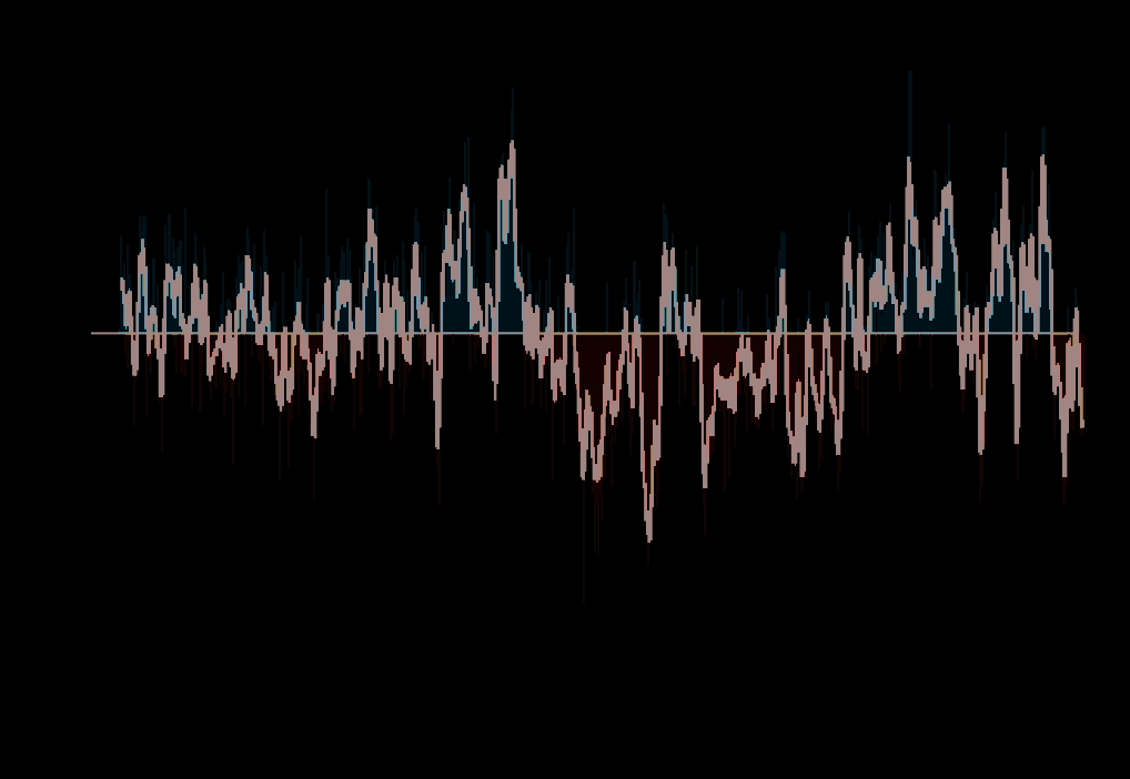
Figure 3À16. a) The North Atlantic Oscillation index from 1860 to
strongly influenced by wind forcing (e.g., Blindheim et
2000 (source: Hurrell, 2002) and b) the Pacific Decadal Oscillation
al., 2000; Hansen et al., 2001; Mork and Blindheim,
index 1900 to 2000.
2000; Orvik et al., 2001), with a large component of
which, together with the shorter transit times, contrib-
variation accounted for by the NAO index (Figure 3À17).
uted to warming by about 2.3░C of the Atlantic water
entering the Arctic Ocean (Swift et al., 1997). The At-
High North Atlantic Oscillation
lantic water also exhibited slightly decreased salinity (by
index
0.03-0.05), probably reflecting increased precipitation in
Barents
Sea
the Nordic Seas during NAO+ conditions (Figure 3À4 b).
Within the Arctic Ocean, the changes in the distribu-
Greenland
Sea
tion and composition of the Atlantic Layer water were
Norwegian
spectacular when set against the traditional perception
Sea
of a quiet, steady-state ocean (see Figures 3À13 and 3À15
Iceland
Sea
for the position of the Atlantic Layer within the water
column). The front between Atlantic water and Pacific
water, traditionally located over the Lomonosov Ridge
Irminger
was forced over to the Alpha-Mendeleev Ridge (Figure
Sea
Labrador
3À13 and see McLaughlin et al., 1996; Morison et al.,
Sea
2000). At the same time, the inflowing water could
be detected in the Atlantic Layer by an approximately
Atlantic water
a
1.5░C temperature rise above the climatological norm
Arctic water
(Carmack et al., 1995). The changes in volume and com-
position of Atlantic water entering the Arctic Ocean
Low North Atlantic Oscillation
through Fram Strait continue to cascade through the
index
Arctic basins, first as changes in properties along the
boundaries (McLaughlin et al., 2002; Newton and So-
tirin, 1997), then as changes propagated into the basin
interiors along surfaces of constant density (Carmack et
al., 1997) (Figure 3À13). Woodgate et al. (2001) esti-
mated that in 1995 to1996, the boundary flow over the
southern margin of the Eurasian Basin was transporting
5 ▒1 Sv at about 1 to 5 cm/s (300 -1600 km/yr). When
water in the boundary current reached the Lomonosov
Ridge, the flow split with around half entering the Cana-
dian Basin along its margin and half returning toward
Fram Strait along the Lomonosov Ridge. The high NAO
index of the late 1980s (Figure 3À16 a) also strengthened
b
and warmed the inflowing Barents Sea branch of At-
lantic water, perhaps by as much as 25% relative to
Figure 3À17. Main features of the circulation of Atlantic waters
1970 (Dickson et al., 2000), which probably led to a
(red) and Arctic waters (blue) in the northern North Atlantic and
parallel warming and increase in salinity of the Barents
Nordic Seas under a) pronounced NAO+ conditions and b) pro-
Sea (Zhang et al., 2000).
nounced NAO ¡ conditions (source: Blindheim et al., 2000).
Recent Change in the Arctic and the Arctic Oscillation
19
Year, NAO
nants. In the Greenland Sea, deep or intermediate water
1960
'65
'70
'75
'80
'85
'90
'95
masses are created by winter cooling of the upper layer,
NAO 4
6░E Long.
a process which has weakened or even ceased since the
winter
index
4
beginning of the 1970s (e.g., B÷nisch et al., 1997). In the
░E
2
Barents Sea, vertical mixing takes place down to 300 m
2░E
in cold years, which means the whole water column is well
0
NAO
mixed from the surface to the bottom. In addition to ver-
0
¡ 2
tical mixing due to cooling in the open sea, vertical mix-
2░W
ing also takes place in frontal zones of the Nordic and Ba-
¡ 4
rents Seas. Cold and warm water masses meet and mix
4░W
to create a very productive area where there is likely to
¡ 6
35 PSU
6░W
be a high organic sedimentation rate. The fronts also act
as a barrier for distribution of both plankton and fish.
¡ 8
8░W
1965 '70
'75
'80
'85
'90
'95
2000
Year, longitude of salinity 35
3.6.2. The Bering and Chukchi Seas
Figure 3À18. A comparison of the western extent of Atlantic Water
The eastern Bering and Chukchi Seas are contiguous
(brown curve) and the NAO index (blue curve). The brown curve
reflects three-year moving averages of the longitude of maximum
shelves that extend nearly 2000 km northward from the
western extent of water with salinity of 35 in the section along
Alaskan Peninsula to the continental slope of the Arctic
65░45'N (source: Blindheim et al., 2000). The blue curve reflects a
Ocean's Canada Basin (Figure 3À19). Both shelves are
three-year moving average of NAO winter values (Dec- March) (up-
broad and shallow with typical depths on the Bering and
dated from Hurrell, 1995). The two lines are strongly correlated
Chukchi shelves being <100m and < 60m, respectively.
with a time-lag of ca. 2-3 years between respective peaks.
The Bering Strait provides a continuous pathway by
A high winter NAO index (December-March) is associ-
which approximately 25 000 km3 of water from the
ated with more south-westerly winds and storms which
North Pacific Ocean enter the Arctic Ocean annually
increase the volume flux of the inner (eastern) branch of
(Roach et al., 1995). The nutrient-rich, but moderately
the NwAC (compare Figure 3À17 a with Figure 3À17 b;
M
Orvik et al., 2001). Under these conditions, more At-
inimum
Beaufort
lantic water reaches the Barents Sea and the Arctic
East
Sea
70░N
Siberian
Ocean, and less Atlantic water is transported into the
Sea
central Norwegian Sea (Blindheim et al., 2000). Coinci-
Chukchi
Sea
dentally, more Arctic water from the East Greenland
Maximum
Current, which is fresher and cooler, enters the central
Norwegian Sea. During periods of low NAO index (Fig-
Siberia
Alaska
ure 3À17 b), weaker south-westerlies result in a weaker 65░N
inner branch of the NwAC and a greater extension of
Atlantic water to the west in the Norwegian Sea. The
east¡west extent of Atlantic water passing through the
Yukon River
M
Norwegian Sea predictably follows the winter NAO
inimum
index with a lag of 2 to 3 years (Figure 3À18).
60░N
Large-scale atmospheric features, as represented by
the NAO, appear to affect the strength of the Atlantic
aximum
M
inflow to the Barents Sea (Figure 3À17; Dippner and Ot-
tersen, 2001; Ingvaldsen et al., 2002) but this inflow
seems also to be closely related to regional atmospheric
Bering Sea
55░N
circulation (┼dlandsvik and Loeng, 1991). Low atmos-
pheric pressure over the inflow area favours increased
Gulf of Alaska
inflow of Atlantic water resulting in higher than average
Aleutian Islands
temperatures in the Barents Sea.
500 km
From the mid-1960s the NAO index has increased
progressively with relatively high values in the early- to
180░W
175░W
170░W
165░W
160░W
155░W
0
Depth, m
mid-1990s (Figure 3À16 a). Increased atmospheric car-
Beaufort Gyre
Siberian Coastal Current
20
bon dioxide (CO
Alaska Coastal Water
2) is projected to increase storm fre-
Bering Shelf Water
100
quencies and weaken thermohaline circulation (IPCC,
Aleutian North Slope ¡ Bering Slope ¡ Anadyr Waters
200
2002) probably producing upper ocean circulation more
Alaskan Stream
September ice edge maximum and minimum extents
1000
like that observed during NAO+ conditions (Figure
March ice edge maximum and minimum extents
7000
3À17 a). The increased wind-induced transport may be
Figure 3À19. A schematic diagram of circulation in the Bering¡
partly compensated for by a reduced thermohaline circu-
Chukchi region of the Arctic. Flow over the Bering Sea shelf consists
lation with the net effect of a relatively large transport of
of waters from the Alaskan Stream, which feeds the Bering Slope
Atlantic water to the Barents Sea and the Arctic Ocean,
Current, and fresher water from the Gulf of Alaska shelf which con-
and increased influence of Arctic water masses on the
tributes to northward transport over the eastern Bering Shelf. In the
Chukchi region, the Siberian Coastal Current transports fresh, cold
western and central Norwegian Seas.
water from the East Siberian Sea. Maximum (March) and minimum
Vertical mixing of water masses is important for bio-
(September) ice coverage and their variations are shown by dashed
logical production and for redistribution of contami-
lines (adapted from NOCD, 1986).
20
AMAP Assessment 2002: The Influence of Global Change on Contaminant Pathways
Water transport, m3/s
100 000
Bering Strait
Roach et al., 1995
80 000
Measured
Coachman and Aagaard, 1988
60 000
Jan-Aug
a
40 000
1950
1960
1970
1980
1990
Total annual precipitation, m
Bering Sea shelf
0.8
St. Paul
0.6
Average
Nome
Figure 3À20. Time series of a) mean
0.4
Average
annual transport of water through
Bering Strait from 1946 to 1996
(adapted from Roach et al., 1995)
and b) precipitation over the Be-
0.2
b
ring Sea shelf based on annual pre-
cipitation measurements.
1950
1960
1970
1980
1990
2000
fresh Pacific inflow plays an important role in stratifying
and Chukchi Seas following atmospheric transport across
the upper 200 m of the Canada Basin (Carmack, 1986;
the North Pacific from Asia (Li et al., 2002; Macdonald
Coachman and Aagaard, 1974) and can be detected as
and Bewers, 1996; Macdonald et al., 2002b; Wilkening
far away as Fram Strait (Jones and Anderson, 1986;
et al., 2000).
Newton and Sotirin, 1997). The freshness of Pacific wa-
Salinity variations of ~1 in the inflowing Pacific water
ters is supported by river runoff onto the Bering Sea
(Roach et al., 1995) correspond to a range in injection
shelf, relatively fresh inflow from the Gulf of Alaska
depth into the Arctic Ocean halocline of 80 m or more,
(Royer, 1982), and greater precipitation than evapora-
which is significant in determining whether, or how, con-
tion over the North Pacific Ocean (Warren, 1983).
taminants from the Pacific Ocean might enter Arctic
Any alteration in the global thermohaline circulation
Ocean food webs. Salinity variation over the Bering shelf
(occurring at time scales of hundreds of years) will prob-
is controlled partly by sea-ice production and melting
ably lead to change in the amount and composition of
and partly by net precipitation, this latter process being,
water passing through Bering Strait (see, for example,
itself, an important pathway for some contaminants
Wijffels et al., 1992). Interannual and decadal scale vari-
(e.g., Li et al., 2002). Precipitation exhibits interannual
ations in water transport, which may account for 40%
variations that are as high as 50% of the long-term aver-
of the variation in the long-term mean, are predomi-
age, and also decadal or longer cycles with, for example,
nantly forced by the regional winds (Figure 3À20 a)
the 1960s to 1970s being relatively dry (Figure 3À20 b).
whose strength and direction depends on the intensity
The ice edge in the Bering¡Chukchi Seas migrates an-
and position of the Aleutian Low (Figure 3À2). Variation
nually as much as 1700 km between the southern Bering
on the decadal scale (water transport was 15% lower
shelf in winter (lowest dashed line on Figure 3À19) to the
during 1973 to 1996 than during 1946 to 1972) has also
northern Chukchi shelf in summer (highest dashed line
been inferred from wind records (Figure 3À20 a).
on Figure 3À19) with interannual variability of as much
Upwelled Pacific waters support one of the world's
as 400 km (Niebauer, 1998; Walsh and Johnson, 1979).
most productive ecosystems in the northern Bering ¡
Variability in ice cover is governed by the strength and po-
southern Chukchi Seas (Springer et al., 1996; Walsh et
sition of the Aleutian Low and East Siberian High (Figure
al., 1989), including both oceanic fauna and shelf fauna
3À2) which influence storm tracks across the North Pa-
transported within the surface water flowing northward
cific (Niebauer, 1998; Overland and Pease, 1982). In the
over the Bering shelf (Walsh et al., 1989). These shelves
Chukchi Sea, the summer and autumn ice edge position
also serve as an important migratory pathway and criti-
can vary by as much as 200 km from its seasonally ad-
cal habitat for a rich and diverse group of marine mam-
justed mean location (NOCD, 1986), with this variabil-
mals, birds, and fish that move between polar, temper-
ity associated with wind anomalies (Maslanik et al.,
ate, and tropical waters (Ainley and DeMaster, 1990;
1999). A significant decrease in ice cover over the Bering
Tynan and DeMaster, 1997).
Sea appears to have coincided with a shift in the late
Pacific waters are substantially modified over the
1970s from the `cold' phase of the Pacific Decadal Oscil-
shelves through exchanges with the land, atmosphere,
lation (PDO) (Figure 3À16 b) to its `warm' phase (Figure
seabed, ice cover, and through biogeochemical transfor-
3À21, and see also Macklin, 2001; Niebauer, 1998).
mations within the water column. These processes,
In the Bering Strait, late summer and autumn water
which vary tremendously on seasonal and interannual
temperatures can exceed 7║C, with substantial year-to-
time scales, affect the fate and distribution of contami-
year variability. This variability, which affects ice melt on
nants deposited in the northeast Pacific and the Bering
the Chukchi shelf and possibly the developmental rates
Recent Change in the Arctic and the Arctic Oscillation
21
Ice concentration, %
ure 3À20 a), therefore, affects ice climate in the Chukchi
80
1972-1976
Sea. Furthermore, variations in summer water properties
a
Cold PDO
and/or transport could lead to changes in the structure
60
of shelf and slope food webs, insofar as the warm water
40
provides suitable seasonal habitat for Pacific organisms
20
advected into the Arctic (Melnikov et al., 2002).
The volume and salinity of dense water formed over
0
the Chukchi shelf each winter is affected by the extent of
40
1977-1989
the seasonal retreat and advance of sea ice, which is vari-
b
Warm PDO, AO¡
20
able and may change with warming. A thin ice cover in
the autumn promotes early cooling of shelf waters, new
0
ice growth, and the formation of multiple high-salinity
100
water mass modes (Figure 3À22 a), whereas thick ice cover
c
Early loss of ice cover
in 2000
80
delays cooling, inhibits new ice growth, and leads to low-
1990-2000
Warm PDO, AO+
salinity water mass modes (Figure 3À22 b). These water
60
masses then exchange differently with the interior ocean.
40
1993-94
32.7-33.1
20
(~150 m)
33.5-33.7
(~175 m)
Number of observations
0
100
Oct Nov Dec Jan Feb Mar Apr May Jun Jul Aug Sep
32.3
a
(75 m)
Figure 3À21. Ice concentration over the southeastern Bering Sea be-
31.3
34.5
(< 50 m)
tween 57░N and 58░N for a) a cold PDO phase (1972-76), b) a warm
(> 250 m)
PDO and an AO ¡ phase (1977¡89), and c) an intermediate regime
with a warm PDO and an AO + phase (1990-2000). Red line shows
50
the early loss of ice cover in 2000 (adapted from Macklin, 2001).
of fish and other marine organisms, is related to change
in large-scale advection and/or the summer radiation bal-
ance over the Bering Sea. Most of the ice in the Bering Sea
grows and melts in situ such that brine rejection and melt-
0
ing strongly influence this shelf's water properties and
31
32
Salinity, PSU
33
1
0
¡1
¡ 2
░C
stratification. During a spring and summer following
34
35
2
3
Temperature,
heavy ice cover, the shelf water column is more strongly
stratified and bottom temperatures are considerably lower
32.7
(Azumaya and Ohtani, 1995), exerting a substantial in-
(100 -150 m)
1994-95
Number of observations
fluence on species composition and the distribution of
300
marine fish, birds, and mammals (Wyllie-Echeverria and
b
Ohtani, 1998; Wyllie-Echeverria and Wooster, 1998).
Ice cover also affects the carbon cycle. In spring,
250
when nutrient concentrations are high, meltwater from
31.5
(< 50 m)
sea ice stratifies the euphotic zone and initiates an ice
edge bloom. Because zooplankton concentrations are
low due to cold water temperatures, ungrazed phyto-
200
plankton settle to the seabed. In the absence of ice, water
temperatures are warmer, phytoplankton are consumed
by zooplankton, and less carbon is delivered to the ben-
150
thos (Niebauer and Alexander, 1985).
Throughout spring and summer, waters of the cen-
tral Bering shelf are strongly stratified owing both to the
100
previous winter's ice history and to summer surface
warming by solar radiation. Wind mixing is required to
erode the stratification and replenish the euphotic zone
50
with nutrients from depth. Springer (pers. comm., 2001.)
shows that there is large interannual variability in wind
speed, which provides the energy for mixing, and wind
0
speeds over the Bering Sea seem to have diminished since
31
32
the late 1970s by ~ 40%, coincident with the shift in the
Salinity, PSU
33
░C
34
1
0
¡1
¡ 2
35
2
3
PDO from its cold phase to its warm phase.
Temperature,
The northward advection of warm water from the
Figure 3À22. Water properties (T, S) on the northeastern Chukchi
Bering Strait causes ice melt to occur earlier over the
shelf in a) 1993-1994, with light autumn ice cover, large polynyas in
Chukchi shelf and freeze-up to be delayed, thereby pro-
winter, and multiple high-salinity water mass modes; and b) 1994-
1999, with heavy autumn ice cover, small polynyas, and low-salin-
longing the ice-free season relative to most other Arctic
ity water mass modes. The depths in parentheses refer to the depth
shelves (Martin and Drucker, 1997; Paquette and Bourke,
to which each mode would sink along the continental slope if no
1981). Variability in flow through the Bering Strait (Fig-
mixing occurred.
22
AMAP Assessment 2002: The Influence of Global Change on Contaminant Pathways
The Siberian Coastal Current (SCC; Figure 3À19),
itself, together with non-uniform spatial distribution of
flowing eastward along the Siberian coast for ~2000
properties including river water and contaminants (e.g.,
km, also contributes low-salinity water to the Chukchi
see Carmack et al., 1997; Guay and Falkner, 1997)
shelf (Coachman et al., 1975; Weingartner et al., 1999).
should indicate the potential for upstream basin changes
From its probable origin in the western East Siberian
to be recorded as variable contaminant loadings in
Sea, the SCC draws water from as far as the Laptev Sea
water flowing through the Archipelago. Furthermore,
including ice melt and river discharges from the Lena,
bowhead whale remains and driftwood on Archipelago
Indigirka, Kolyma and other Russian rivers along the
shores suggest that ice-drift trajectories and ice cover
way (Figure 1À1, Proshutinsky et al., 1995). Zooplank-
have both varied greatly over time (Dyke et al., 1996b,
ton aggregate along the front between the SCC and the
1997; Dyke and Savelle, 2000, 2001) implying that the
warmer, saltier water flowing through Bering Strait, pro-
Canadian Arctic Archipelago is sensitive to rapid and
viding important feeding opportunities for bowhead
dramatic change.
whales (Balaena mysticetus) in the western Chukchi Sea
(Moore et al., 1995) and potentially a critical pathway
3.6.4. Hudson Bay
for contaminants to enter the food web at that point. Al-
though transport in the SCC is relatively small (~3000
Hudson Bay is a large, shallow, semi-enclosed sea
km3/yr), its low-salinity waters enriched by runoff from
strongly influenced by seasonal runoff. The annual dis-
Russian rivers could substantially dilute the inflow
charge (710 km3/yr) is equivalent to a freshwater yield of
through Bering Strait and influence the distribution of
about 65 cm (Prinsenberg, 1991). Presently, this sea ex-
Pacific waters in the Arctic Ocean.
hibits a complete cryogenic cycle with summer (August-
The SCC exemplifies several ways in which changes
October) being ice free and winter fully ice covered. Cli-
in Arctic coastal currents can affect the transport and
mate models suggest that a doubling of CO2 may lead to
dispersal of contaminants (dissolved or sediment-bound).
the virtual disappearance of ice from Hudson Bay there-
Firstly, coastal currents have large seasonal variability
by raising winter air temperatures and leading to the
because 75 to 90% of the river discharge occurs within a
thawing of permafrost in adjacent land areas (Gough
three-month summer period. Change in the timing or
and Wolfe, 2001). These same models predict that the
amount of freshwater inflow will be expressed in the
complete loss of ice will be preceded by years exhibiting
seasonal structure of the shelf circulation (Omstedt et
earlier break-up and later freeze-up. According to Stir-
al., 1994). Secondly, coastal currents provide a vector to
ling and co-workers (1999), some of these projected
transport contaminants along a vast shoreline that can
23 Aug
be dramatically altered by windfield change accompany-
ing the AO (see Figure 3À14, section 3.5.2.1 and Guay et
13 Aug
Mean ashore date
al., 2001; Johnson and Polyakov, 2001; Weingartner et
of polar bears
3 Aug
al., 1999). Thirdly, river ice breakup typically occurs be-
fore the landfast ice melts with the result that little mix-
24 Jul
ing initially occurs between the river water and the am-
14 Jul
bient shelf water and the inner shelf becomes strongly
Date of ice break-up
stratified (Ingram, 1981; Macdonald et al., 1995). After
04 Jul
the landfast ice melts, plume behaviour depends criti-
24 Jun
cally on the time-integrated effects of the wind velocity.
Under `upwelling' favourable winds, freshwater plumes
14 Jun
can easily spread to interior basins carrying contami-
1991
1992
1993
1994
1995
1996
1997
1998
nants far beyond the shelf break (Macdonald et al.,
Figure 3À23. Temporal trends in the date of ice break up and the
1999a). Under `downwelling' favourable winds coastal
mean date at which polar bears return to shore in Hudson Bay. The
currents are more likely to be formed (Melling, 1993;
break-up dates refer to that region in Hudson Bay where satellite-
tagged female polar bears spent at least 90% of their time (modified
Weingartner et al., 1999). Lastly, the dispersal and stor-
from Stirling et al., 1999).
age of freshwater over Arctic shelves in late summer set
limits on the density of water that can be formed by sea-
changes may already be occurring (Figure 3À23), putting
ice production the following winter (Macdonald, 2000;
considerable stress on the western Hudson Bay polar
Melling, 1996; Weingartner et al., 1999).
bear (Ursus maritimus) population.
The hydrological cycle of Hudson Bay has been
strongly altered through immense damming projects in
3.6.3. The Canadian Arctic Archipelago
the drainage basin, leading to an increase in winter
The Canadian Arctic Archipelago provides one of the
runoff to Hudson Bay of over 50% (Prinsenberg, 1991).
important outlets for Arctic Ocean surface water (Figure
Not only do such changes have an impact on stratifica-
1À1). Therefore, both changes in Arctic Ocean surface
tion and hence nutrient cycling in this sea, but newly-
water contaminant burdens and changes in the source of
flooded reservoirs are well known for their secondary ef-
water flowing out through the Archipelago have the po-
fect of releasing mercury to downstream aquatic envi-
tential to alter contaminant concentrations within the
ronments (Bodaly and Johnston, 1992).
Archipelago's channels. There are few data with which
Due to its southern location, Hudson Bay is clearly
to evaluate how seawater within the Archipelago chan-
in the vanguard of Arctic change and is, therefore, a vital
nels responds to the AO. However, changes in distribu-
region to collect time series. According to Figure 3À3 a,
tion of surface water properties (Figures 3À13 and 3À14)
Hudson Bay lies on a divide between warming and cool-
and ice drift trajectories (Figure 3À9) in the Arctic Ocean
ing. Regional temperature maps and other evidence
Recent Change in the Arctic and the Arctic Oscillation
23
(Gilchrist and Robertson, 2000; Skinner et al., 1998)
a receptor through snow fall in winter, and a conveyor
confirm that between 1950 and 1990, the western side
through runoff in spring. From a very limited set of stud-
has warmed at about the same rate as the eastern side
ies, it appears that Arctic lakes presently retain only a
has cooled. In agreement with this observation, bears on
small fraction of contaminant inputs because the main
the eastern side of Hudson Bay do not show the same
runoff pulse, which precedes lake turnover and peak pri-
pattern of weight loss as the bears on the western side
mary production, simply traverses the lake surface under
(Stirling et al., 1999), further emphasizing the impor-
the ice (Macdonald et al., 2000a). With lakes exhibiting
tance of this region as a laboratory to study detailed
more temperate characteristics, the coupling of runoff
consequences of change by contrast.
with lake mixing and primary production will change,
probably allowing lakes to capture more of the inflow-
ing contaminant burden. In particular, the potential for
3.6.5. Baffin Bay, Davis Strait and the Labrador Sea
snow surfaces to enhance contaminant fugacity in lake
Baffin Bay, Davis Strait and the Labrador Sea occupy a
settings is extremely large (Macdonald et al., 2002c).
unique position in that they may receive contaminants
However, quantitative measurements of contaminant¡
both from ice and water that exit the Arctic Ocean in the
snow interactions are required because the significance
East Greenland Current and also from water and ice
of snow in contaminant cycling cannot be projected sim-
passing through the Canadian Arctic Archipelago.
ply from hydrological measurements.
Change, therefore, can be produced by variation of con-
taminant composition within either of these sources or
3.8. Permafrost
by altering their relative strength and the strength of
direct exchange with the atmosphere. Furthermore,
Permafrost underlies about 25% of the land in the
decadal-scale modulation probably differs for the vari-
Northern Hemisphere, including large areas of Canada,
ous sources, with the AO perhaps influencing Archipel-
Russia, China and Alaska (Figure 3À24, Zhang et al.,
ago through-flow or Fram Strait outflow, whereas the
1999). Permafrost can also be found in sediments of the
ice cover in Baffin Bay is more closely associated with
continental shelves (not shown). Especially vulnerable to
the Southern Oscillation (Newell, 1996). In agreement
change are regions of discontinuous permafrost which
with spatial temperature patterns (Figure 3À3 a), whereas
include large parts of northern Canada, Alaska and Rus-
ice season has been getting shorter within the Arctic
sia. The IPCC (2002) suggests that permafrost area
Ocean and its marginal seas, Davis Strait and the Lab-
could be reduced by 12 to 22% by 2100 with perhaps as
rador Sea have recently exhibited an increase in the
much as half of the present-day Canadian permafrost
length of ice season (Parkinson, 1992).
disappearing.
Long-period cycles in the ice climate of this region
In regions of permafrost, the active layer of soil, typ-
(50 years or more) appear to have had dire consequences
ically limited to the top 1 m, supports almost all of the
for both terrestrial and marine biological populations ¡
biological processes. The loss of permafrost, therefore,
including humans (Vibe, 1967). Like Hudson Bay, this
alters these biological processes, including affecting the
appears to be an important region to study in the con-
kind of vegetation that can grow, and changes the way
text of contaminants (Fisk et al., 2001a), biogeographi-
soil interacts with the hydrological cycle (Osterkamp et
cal variation (Johns et al., 2001) and the impact of
al., 2000; V÷r÷smarty et al., 2001) both of which have
change on humans (Woollett et al., 2000). Furthermore,
consequences for contaminant transport. In particular,
surface water from Baffin Bay is exported to the south
thawing frozen ground releases sediment, nutrients, and
via Davis Strait to feed the Labrador Current (along
with outflow from Hudson Bay and the Canadian Arctic
Archipelago ¡ Figure 1À1). Baffin Bay, therefore, pro-
Permafrost distribution
vides a region of transition which can export change in
ocean properties (freshwater, contaminants, biota) to
the Northwest Atlantic.
3.7. Lake and river ice
Arctic lakes and rivers are likely to provide sensitive sen-
tinels of climate change in their freeze, melt and hydro-
logical cycles (V÷r÷smarty et al., 2001). Whereas there
appear to be no studies showing a relationship between
freshwater ice cover and the AO, significant trends in
these properties over the past 150 to nearly 300 years
have been demonstrated (Magnuson et al., 2000; Semile-
tov et al., 2000). During the period between 1846 and
1995, there has been a mean delay of 5.8 days per cen-
tury for freeze-up and a corresponding 6.5 days per cen-
Continuous
Discontinuous
tury advance in break-up. This change in the freeze/melt
Sporadic
cycle implies increasing temperatures of about 1.2░C per
Isolated
century.
Most Arctic lakes receive their contaminant burdens
Figure 3À24. The distribution of permafrost in northern landmasses
from the atmosphere, with the catchment area acting as
(source: IPA, 2001).
24
AMAP Assessment 2002: The Influence of Global Change on Contaminant Pathways
organic carbon which then enter ground water, rivers
Glacial melt, km3
and lakes to impact upon biological cycles (see, for ex-
50
Canada
ample, the studies done in the Mackenzie Basin; Cohen,
1997a). The observed thawing trends in Alaska and
Russia, but not in northeastern Canada, appear to match
0
the observed trends in SAT (see Figure 3À3 a and Rigor et
al., 2000). Accelerated permafrost degradation during
the 1990s can probably be ascribed at least partly to the
¡ 50
AO (Morison et al., 2000) with, for example, the advec-
tion of warm air into the Russian Arctic during strong
AO+ conditions contributing to thawing in that region.
¡100
In addition to the changes in biogeochemical path-
ways that will accompany permafrost degradation, there
will also be the widespread problem of re-mobilization
¡150
of contaminants (see, for example, conference proceed-
ings dedicated to the issue of contaminants in frozen
¡200
ground; Anon., 2001a,b). Historical disposal of waste
1965
1970
1975
1980
1985
1990
1995
substances has occurred in the form of sewage lagoons,
dump sites at DEW line sites (Distant Early Warning
Figure 3À25. The loss of glacial ice mass, km3/yr, in the Canadian
Arctic between 1961 and 1993 based on data compiled by Serreze
Line; a chain of defense radar stations, many now aban-
et al. (2000) and Dyurgerov and Meier (1997).
doned, along 66░N in Canada, also extending into
Alaska and Greenland), solid waste dumps in small Arc-
tions, at a rate of about 51 km3/yr (Krabill et al., 2000).
tic communities, mine tailings, and oil drilling sumps.
Data also point clearly to loss of ice mass for small gla-
A large component of the containment strategy for these
ciers in the Arctic during the interval between 1961 and
sites is the presence of permafrost. With permafrost
1993 (Arendt et al., 2002; Dyurgerov and Meier, 1997;
degradation, landfills can become washed directly into
Serreze et al., 2000). Since about 1960, glacial melt-back
rivers or the ocean, or runoff can leach contaminants
in the Canadian Arctic alone (Figure 3À25) is estimated
into local groundwater. In locations such as river deltas
at over 800 km3 ¡ around half of the melt-back esti-
and coastal plains, low relief may provide a shortcut be-
mated for the whole Arctic (Dyurgerov and Meier,
tween such waste sites and drinking water.
1997). In conformity with the strong AO+ conditions of
the early 1990s, the loss of glacial ice mass in the Cana-
dian Arctic Archipelago was exceptionally strong in the
3.9. Glacial ice
early 1990s, amounting to 390 km3 (Figure 3À25).
Most Arctic glaciers have experienced net loss in ice
Glaciers may act as long-term reservoirs, sequester-
mass over the past few decades (Dowdeswell et al.,
ing and preserving airborne contaminants during peak
1997). The Greenland ice mass appears presently (1994-
emission years (1950-1970) later to release them during
1999) to be decreasing, predominantly at lower eleva-
periods of melt-back (Blais et al., 1998).