Appendix 1
Federated States of Micronesia --
Climate Risk Profile
Summary
unit, information is often insufficient to assess this
spatial variability, or the variations are judged to be
of low practical significance.
The likelihood (i.e., probability) components The following climate conditions are consid-
of climate-related risks in the Federated
ered to be among the potential sources of risk:
States of Micronesia (FSM) are evaluated, for
both present-day and future conditions.
·
extreme rainfall events,
Changes over time reflect the influence of global
·
drought,
warming.
·
high sea levels,
The risks evaluated are extreme rainfall events
·
strong winds, and
(both hourly and daily), drought, high sea levels,
·
extreme high air temperatures.
strong winds, and extreme high air temperatures.
Projections of future climate-related risk are
B.
Methods
based on the output of global climate models, for
given emission scenarios and model sensitivity.
With the exception of maximum wind speed,
Preparation of a climate risk profile for a given
projections of all the likelihood components of
geographical unit involves an evaluation of current
climate-related risk show marked increases as a
likelihoods of all relevant climate-related risks,
result of global warming.
based on observed and other pertinent data.
Climate change scenarios are used to develop
projections of how the likelihoods might change in
A. Introduction
the future. For rainfall and temperature projections,
the Hadley Centre (United Kingdom) global climate
Formally, risk is the product of the consequence
model (GCM) was used, as it gave results interme-
of an event or happening and the likelihood (i.e.,
diate between those provided by three other GCMs,
probability) of that event taking place.
namely those developed by the Australian Com-
While the consequence component of a
monwealth Scientific and Industrial Research
climate-related risk will be site or sector specific, in
Organisation, Japan's National Institute for Environ-
general the likelihood component of a climate-
mental Science, and the Canadian Climate Centre.
related risk will be applicable over a larger
For drought, strong winds, and sea level, the Cana-
geographical area and to many sectors. This is due
dian GCM was used to develop projections.
to the spatial scale and pervasive nature of weather
Similarly, the SRES A1B greenhouse gas
and climate. Thus the likelihood of, say, an extreme
emission scenario was used when preparing rainfall,
event or climate anomaly is often evaluated for a
temperature, and sea level projections. Figure A1.1
country, state, small island, or similar geographical
shows that this scenario is close to the middle of the
unit. While the likelihood may well be within a given
envelope of projected emissions and greenhouse
Appendix 1
121

---

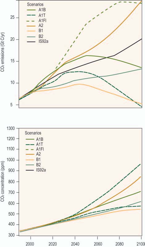
gas concentrations. For drought both the A2 and B2
C.
Information Sources
emission scenarios were used, while for strong
winds only the A2 scenario was used.
Daily and hourly rainfall, daily temperatures,
and hourly wind data were obtained through the
Pohnpei Weather Service Office and with the
assistance of Mr. Chip Guard, National Oceanic and
Figure A1.1. Scenarios of CO Gas Emissions and
2
Atmospheric Administration, Guam. Sea-level data
Consequent Atmospheric Concentrations of CO2
for Pohnpei were supplied by the National Tidal
Facility, The Flinders University of South Australia,
and are copyright reserved. The sea-level data
(a) CO emmisions
2
derived from Topex-Poisidon satellite observations
were obtained from www.//podaac-esip.jpl.nasa.gov.
D. Data Specifications
While much of the original data was reported
in Imperial units, all data are presented using System
International units.
E.
Uncertainties
The sources of uncertainty in projections of the
likelihood components of climate-related risks are
(b) CO concentrations
numerous. They include uncertainties in green-
2
house gas emissions and those arising from model-
ing the complex interactions and responses of the
atmospheric and ocean systems. Figure A1.2 shows
how uncertainties in greenhouse gas emissions
impact on estimates of the return periods of a daily
precipitation of at least 250 mm for Pohnpei.
Similar graphs can be prepared for other GCMs
and extreme events, but are not shown here. Policy
and decision makers need to be cognizant of
uncertainties in projections of the likelihood
components of extreme events.
F.
Graphical Presentations
Many of the graphs that follow portray the
Notes: CO = carbon dioxide; Gt C/yr = gigatonnes of carbon per year.
2
likelihood of a given extreme event as a function of
Source: IPCC 2001.
a time horizon. This is the most appropriate and
useful way in which to depict risk since design life
(i.e., time horizon) varies depending on the nature
of the infrastructure or other development project.
122
Climate Proofing: A Risk-based Approach to Adaptation

---

G. Extreme Rainfall Events
Figure A1.2. Return Periods for Daily Rainfall of
250 mm in Pohnpei for Given Greenhouse
Daily Rainfall
Gas Emission Scenarios
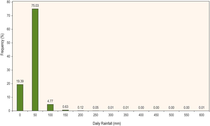
Figure A1.3 shows the frequency distribution of
daily precipitation for Pohnpei. A daily total above
250 mm is a relatively rare event, with a return
period (i.e., recurrence interval) of 10 years.
Figure A1.4 shows the likelihood of such an
extreme rainfall event occurring in Pohnpei and
Kosrae, within a given time horizon ranging from 1
to 50 years.
As shown in Table A1.1, global warming will
significantly alter the return periods, and hence the
likelihoods, of the extreme rainfall events. For
example, Figure A1.5 illustrates how the likelihood
Note: Calculations used Hadley Center GCM with Best Judgment of Sensitivity.
of a daily rainfall of 250 mm will increase over the
Source: CCAIRR findings.
remainder of the present century.
Figure A1.3. Frequency Distribution of Daily Precipitation for Pohnpei
(1953­2003)
mm = millimeters.
Note: The numbers above the bars represent the frequency of occurrence, in percentages, for the given data interval.
Source: CCAIRR findings.
Appendix 1
123

---

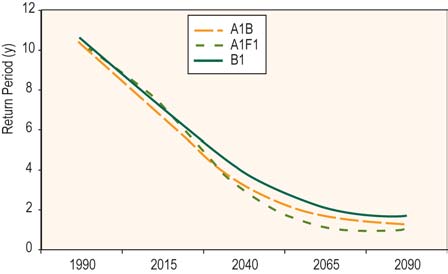
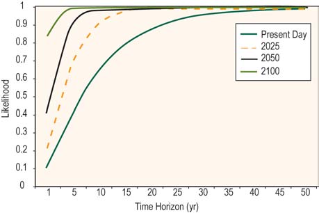
Figure A1.4. Return Periods for a Daily Rainfall
Figure A1.5. Likelihood of a Daily Rainfall
of 250 mm Occurring Within the
of 250 mm Occurring Within the
Indicated Time Horizon
Indicated Time Horizon
(years)
(years)
Note: 0 = zero chance; 1 = statistical certainty.
Data are for Pohnpei (1953­2003) and Kosrae (1953­2001, with gaps). A daily
Note: 0 = zero chance; 1 = statistical certainty.
rainfall of 250 mm has a return period of 10 and 16 years, respectively.
Data are for Pohnpei.
Source: CCAIRR findings.
Source: CCAIRR findings.
Hourly Rainfall
Table A1.1: Return Periods for Daily Rainfall,
Pohnpei and Kosrae
Figure A1.6 shows the frequency distribution of
(years)
hourly precipitation for Pohnpei. An hourly total
above 100 mm (3.9 in) is a relatively rare event. Table
Rainfall
Present
2025
2050
2100
A1.2 shows that such a rainfall has a return period
(mm)
of 6 years. The table also shows, for both Pohnpei
and Kosrae, that global warming will have a
Pohnpei
significant impact on the return periods of extreme
100
1
1
1
1
rainfall events.
150
2
1
1
1
200
5
2
1
1
Figure A1.7 depicts the impact of global
250
10
5
2
1
warming on the likelihood of an hourly rainfall of
300
21
9
4
2
200 mm for Pohnpei.
350
40
17
8
2
400
71
28
13
3
450
118
45
20
5
500
188
68
30
7
H. Drought
Kosrae
Figure A1.8 presents, for Pohnpei, the number
100
1
1
1
1
150
3
2
1
1
of months in each year (1953­2003) and each decade
200
6
4
2
2
for which the observed precipitation was below the
250
16
9
5
2
fifth percentile. Monthly rainfall below the fifth
300
38
21
12
4
350
83
50
31
9
percentile is used here as an indicator of drought.
400
174
119
83
22
Most of the low rainfall months are concentrated
450
344
278
237
64
in the latter part of the period of observation,
00
652
632
410
230
indicating that the frequency of drought has
Source: CCAIRR findings.
increased since the 1950s. The years with a high
124
Climate Proofing: A Risk-based Approach to Adaptation

---

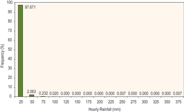
Figure A1.6. Frequency Distribution of Hourly Precipitation for Pohnpei
Notes: Data are for 1980 to 2002, with gaps. The numbers above the bars represent the frequency of
occurrence for the given data interval, in percent of hours of observed rainfall.
Source: CCAIRR findings.
Table A1.2: Return Periods for Hourly Rainfall,
Pohnpei and Kosrae
Figure A1.7. Likelihood of an Hourly Rainfall
(years)
of 200 mm Occurring in Pohnpei Within the
Indicated Time Horizon
(years)
Rainfall
Present
2025
2050
2100
(mm)
Pohnpei
50
2
1
1
1
100
6
3
2
1
150
14
7
4
2
200
23
12
7
4
250
34
18
11
5
300
47
25
15
8
350
61
32
20
10
400
77
40
26
13
Kosrae
50
2
2
1
1
100
8
6
5
3
150
16
13
10
6
Notes: 0 = zero chance; 1 ­ statistical certainty. Values for present day based on
200
28
21
16
11
observed data for 1980­2002, with gaps.
250
41
31
24
16
Source: CCAIRR findings.
300
56
42
33
22
350
73
55
43
29
400
91
68
54
37
Source: CCAIRR findings.
Appendix 1
125

---

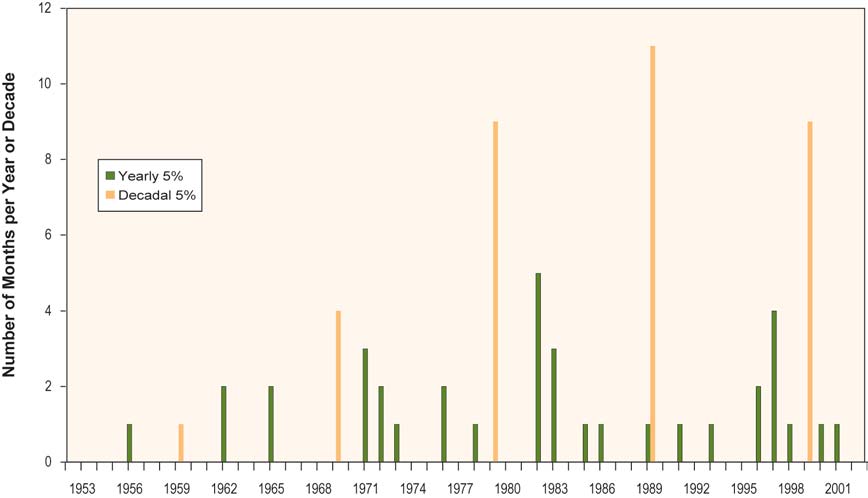
Figure A1.8. Number of Months in Each Year or Decade for Which the
Precipitation Was Below the Fifth Percentile
Note: Data are for Pohnpei.
Source: CCAIRR findings.
number of months below the fifth percentile
I.
High Sea Levels
coincide with El Niņo Southern Oscillation (ENSO)
events.
Figure A1.10 shows daily mean values of sea
A similar analysis could not be undertaken for
level for Pohnpei, relative to mean sea level. Large
Kosrae, because its rainfall records are incomplete.
interannual variability occurs in sea level. Low sea
Figure A1.9 shows the results of a similar
levels are associated with El Niņo events, while
analysis, but for rainfall estimates (1961­1990) and
exceptionally high sea levels occurred in October
projections (1991­2100) by the Canadian GCM. The
1988.
results are presented for both the A2 and B2
Even more extreme high sea levels occur over
emission scenarios.
time scales of less than a day. Table A1.3 provides
Figure A1.9 also shows that the GCM replicates
return periods for given sea level elevations for
the increased frequency of months with extreme low
Pohnpei, for the present day and projected future.
rainfall during the latter part of the last century. The
The latter projections are based on the Canadian
results also indicate that, regardless of which
GCM 1 GS and the A1B emission scenario.
emission scenario is used, the frequency of low
rainfall months will generally remain high relative
to the latter part of the last century.
126
Climate Proofing: A Risk-based Approach to Adaptation

---

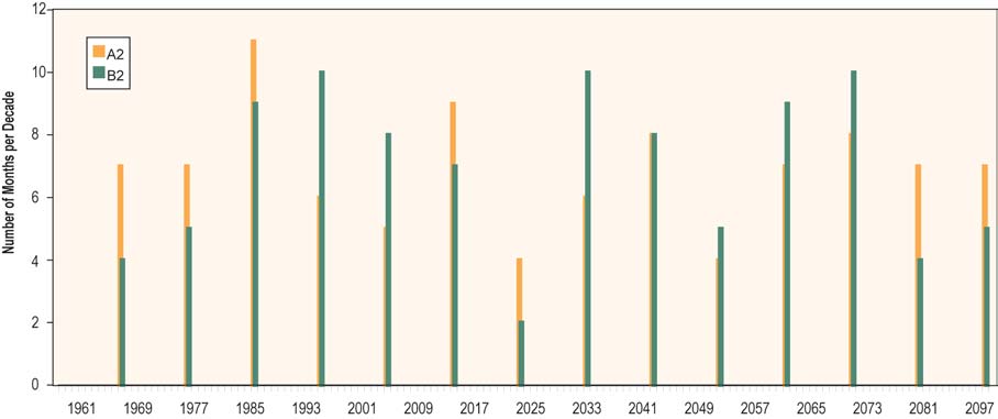
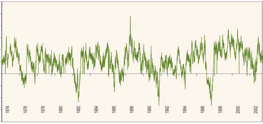
Figure A1.9. Number of Months per Decade for Which Pecipitation for
Pohnpei is Projected to be Below the Fifth Percentile
Note: data from the Canadian Global Climate Model, with A2 and B2 emission scenarios and best estimate for GCM sensitivity.
Source: CCAIRR findings.
Figure A1.10: Daily Mean Values of Sea Level for Pohnpei
(1974­2003)
600
500
400
300
200
100
Sea Level (mm)
0
-100
-200
-300
-400
Note: The sea level elevations are relative to surveyed mean sea level.
Source: CCAIRR findings.
Appendix 1
127

---

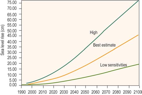
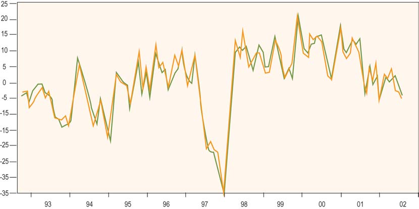
Table A1.3. Return Periods for Extreme
High Sea Levels, Pohnpei
Figure A1.11 Sea-Level Projections for Pohnpei,
(years)
Based on the Canadian GCM 1GS and the
A1B Emission Scenario
Sea Level
Present
2025
2050
2100
(mm)
Day
80
1
1
1
1
90
1
1
1
1
100
4
2
1
1
110
14
5
2
1
120
61
21
5
1
130
262
93
20
1
140
1,149
403
86
2
Note: cm = centimeters.
Source: CCAIRR findings.
The indicated increases in sea level over the
next century are driven by global and regional
cm = centimeters; GCM = global climate model. Uncertainties related to GCM
changes in mean sea level as a consequence of
sensitivity are indicated by the blue, red, and green lines, representing high,
global warming. Figure A1.11 illustrates the
best estimate, and low sensitivities, respectively.
magnitude of this contribution.
Source: CCAIRR findings.
Sea level elevations are not recorded in situ for
Kosrae. However, satellite observations of sea levels
A high level of agreement occurs between the
are available and can add some understanding to
tide gauge and satellite measurements of sea level,
both historic and anticipated changes in sea levels.
at least for monthly averaged data (Figure A1.12).
Figure A1.12. Sea Level (departure from normal) as Determined by the
Pohnpei Tide Gauge and by Satellite
cm
Pohnpei Tide Gauge vs. T/P Altimeter
rms = 2.0 cm
rms = root mean square.
Source: CCAIRR findings..
128
Climate Proofing: A Risk-based Approach to Adaptation

---

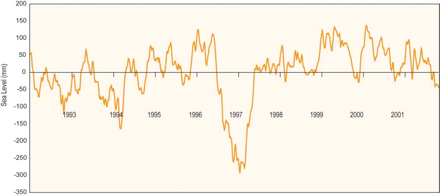
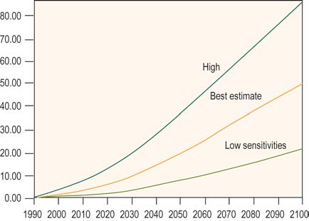
Figure A1.13. Five-Day Mean Values of Satellite-Based Estimates of Sea Level for a Grid Square
Centered on Kosrae (5.25° to 5.37°N; 162.88° to 163.04°E)
Note: Values are departures from the mean for the period of record: November 1992­August 2002.
Source: CCAIRR findings.
This reinforces confidence in the use of satellite
data to characterize sea level for Kosrae. Figure A1.13
Figure A1.14. Sea-Level Projections for Kosrae,
presents satellite-based estimates of sea level for a
Based on the Canadian GCM 1 GS and the
grid square centred on Kosrae.
A1B Emission Scenario
Figure A1.14 presents the projected increase in
sea level for Kosrae as a consequence of global
warming. The global and regional components of
sea-level rise for Kosrae are very similar to those for
Pohnpei.
J.
Strong Winds
Figure A1.15 shows the annual maximum wind
gust recorded in Pohnpei for the period 1974­2003.
Table A1.4 presents return periods for extreme
high winds in Pohnpei, based on observed data. Also
shown are return periods for 1990­2020 and for
2021­2050. The latter are estimated from projections
cm = centimeters; GCM = global climate model. Uncertainties related to GCM
of maximum wind speed using the Canadian GCM
sensitivity are indicated by the blue, red, and green lines, representing high,
2 with the A2 emission scenario.
best estimate, and low sensitivities, respectively.
Source: CCAIRR findings.
Appendix 1
129

---

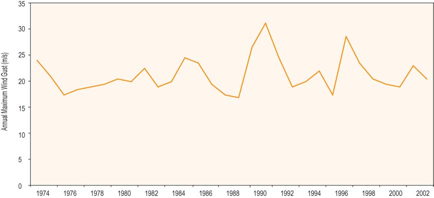
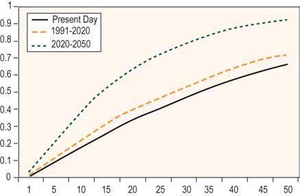
Figure 1.15. Annual Maximum Wind Gust Recorded in Pohnpei for the Period 1974­2003
Note: m/s = meters per second.
Source: CCAIRR findings.
Table A1.4. Return Periods for Maximum
Wind Speed, Pohnpei
Figure A1.16 Likelihood of a Maximum Wind
(years)
Gust of 28 ms-1 Occurring Within the
Indicated Time Horizon in Pohnpei
Wind Speed
Hourly
Daily
(years)
(ms-1)
1974­2003
1961­1990 1991­2020
2021­2050
20
2
2
2
2
25
8
10
10
9
28
20
47
40
20
Source: CCAIRR findings.
Likelihood
Figure A1.16 depicts the impact of global
warming on the likelihood of a maximum wind gust
of 28 ms-1 for Pohnpei.
K. Extreme High Temperatures
0 = zero chance; 1 ­ statistical certainty.
Note: Values based on Canadian Global Climate Model 2, with A2 emission
scenario.
Figure A1.17 presents the frequency distribu-
Source: CCAIRR findings.
tion of daily maximum temperature for Pohnpei.
130
Climate Proofing: A Risk-based Approach to Adaptation

---

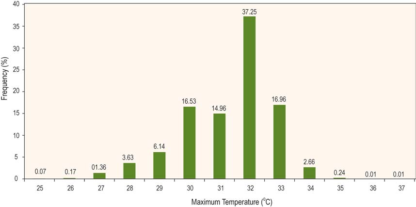
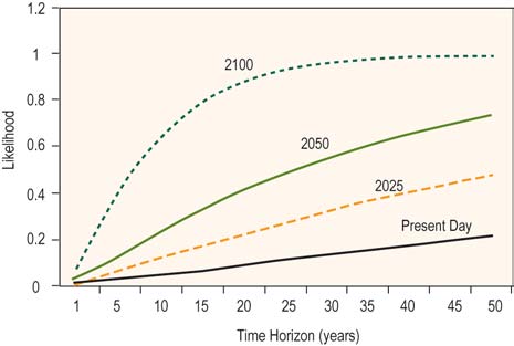
Figure A1.17. Frequency Distribution of Daily Maximum Temperature for Pohnpei
Source: Based on observed data 1953­2001.
Table A1.5 details the return periods for daily
maximum temperature for Pohnpei, based on
Figure A1.18. Likelihood of a Maximum
observed data (1953­2001) and projections using
Temperature of 36°C Occurring Within the
the Hadley Centre GCM and the A1B emission
Indicated Time Horizon in Pohnpei
scenario.
(years)
Figure A1.18 depicts the impact of global
warming on the likelihood of a daily maximum
temperature of 36°C for Pohnpei.
Table A1.5. Return Periods for Daily Maximum
Temperature, Pohnpei
(years)
Maximum
Observed
Projected
Temperature
(1953­2001)
2025
2050
2100
(°C)
32
1
1
1
1
33
1
1
1
1
34
4
2
2
1
35
24
11
6
2
Likelihood 0 = zero chance; 1 ­ statistical certainty.
Notes: Values based on observed data (1953­2001) and on projections from
36
197
80
39
10
the Hadley Centre Global Climate Module (GCM) with A1B emission scenario
37
2,617
1,103
507
101
and best estimate of GCM sensitivity.
Source: CCAIRR findings.
Source: CCAIRR findings.
Appendix 1
131

---