The Regional Organization for the
Conservation of the Environment of
the Red Sea and Gulf of Aden
(PERSGA)
Standard Survey Methods
for Key Habitats and Key Species
in the Red Sea and Gulf of Aden
PERSGA Technical Series No. 10
June 2004

---

PERSGA is an intergovernmental organisation dedicated to the conservation of coastal and marine
environments and the wise use of the natural resources in the region.
The Regional Convention for the Conservation of the Red Sea and Gulf of Aden Environment (Jeddah
Convention) 1982 provides the legal foundation for PERSGA. The Secretariat of the Organization was formally
established in Jeddah following the Cairo Declaration of September 1995. The PERSGA member states are
Djibouti, Egypt, Jordan, Saudi Arabia, Somalia, Sudan, and Yemen.
PERSGA, P.O. Box 53662, Jeddah 21583, Kingdom of Saudi Arabia
Tel.: +966-2-657-3224. Fax: +966-2-652-1901. Email: persga@persga.org
Website: http://www.persga.org
'The Standard Survey Methods for Key Habitats and Key Species in the Red Sea and Gulf of Aden' was prepared
cooperatively by a number of authors with specialised knowledge of the region. The work was carried out
through the Habitat and Biodiversity Conservation Component of the Strategic Action Programme for the Red
Sea and Gulf of Aden, a Global Environment Facility (GEF) project implemented by the United Nations
Development Programme (UNDP), the United Nations Environment Programme (UNEP) and the World Bank
with supplementary funding provided by the Islamic Development Bank.
© 2004 PERSGA
All rights reserved. This publication may be reproduced in whole or in part and in any form for educational or
non-profit purposes without the permission of the copyright holders provided that acknowledgement of the
source is given. PERSGA would appreciate receiving a copy of any publication that uses this material as a
source. This publication may not be copied, or distributed electronically, for resale or other commercial purposes
without prior permission, in writing, from PERSGA.
Photographs: Abdullah Alsuhaibany, Birgit Eichenseher, Gregory Fernette, Fareed Krupp, Hunting Aquatic
Resources, Hagen Schmid, Mohammed Younis
Cetacean illustrations: Alessandro de Maddalena
This publication may be cited as:
PERSGA/GEF 2004. Standard Survey Methods for Key Habitats and Key Species in the Red Sea and Gulf of
Aden. PERSGA Technical Series No. 10. PERSGA, Jeddah.

---

FOREWORD
PERSGA took the initiative during the execution of the Strategic Action Programme for the
Red Sea and Gulf of Aden (SAP) to consider the importance of conserving regional habitats and
biodiversity. The Habitats and Biodiversity Conservation (HBC) component of the SAP developed
a strategy that contained five clear steps: (i) develop a set of standard survey methods (SSMs) for
the region, (ii) train national specialists to use these methods, (iii) execute regional surveys, (iv)
prepare conservation plans, and (v) implement the plans.
In order to evaluate and monitor the status of marine habitats and biodiversity within the Red
Sea and Gulf of Aden, surveys must be undertaken that are comparable in extent, nature, detail and
output. Standardising survey methodology within the region is essential to allow valid comparison
of data, and for the formulation of conservation efforts that are regionally applicable.
The preparation of this guide to the Standard Survey Methods for Key Habitats and Key
Species in the Red Sea and Gulf of Aden was initiated following a review of the methods currently
in use around the world. Contextual SSMs were then drafted for each of the relevant fields: sub-
tidal, coral reefs, seagrass beds, inter-tidal, mangroves, as well as for important groups such as reef
fish, marine mammals, marine turtles and seabirds. The SSM guide was discussed at a regional
workshop in September 2000 held in Sharm el-Sheikh where scientists from both inside and
outside the region reviewed the first drafts and provided the authors with useful comments.
During 2001 PERSGA conducted a series of training courses for regional specialists to teach
them some of these specific methods. The training courses were also used as tools to evaluate the
methods and to determine their applicability to our region. The results of the evaluations given by
the specialists recognized the suitability of these SSMs for our region due to a combination of
factors: their widespread use, their simplicity and the particular adaptations made to suit the region.
We are proud to provide our region with this SSM guide. It has been recognized by experts
from all over the world and tested by regional specialists. We hope this guide can be improved
upon in the future and will play its part in achieving the goal of sustainable development of marine
and coastal resourses in the region.
This guide will form an important tool to be used by management to help make decisions that
will prevent an otherwise irreversible decline in the status of our marine habitats and species.
Dr. Abdelelah A. Banajah
Secretary General PERSGA
i

---

ACKNOWLEDGEMENTS
This document was prepared by PERSGA through the Habitat and Biodiversity Component of the Strategic
Action Programme for the Red Sea and Gulf of Aden (SAP). Due acknowledgement is accorded to the GEF
Implementing Agencies (UNEP, UNDP, the World Bank) and the Islamic Development Bank for financial and
administrative support. Our sincere thanks go to all the authors and illustrators who contributed to the preparation
of this document.
Several regional specialists are thanked for the significant contribution they made to the completion of this
document. They are: Dr. Nabil Mohamed (Djibouti), Dr. Mohamed Abou Zaid (Egypt), Dr. Salim Al-Moghrabi
(Jordan), Dr. Abdul Mohsen Al-Sofyani (Saudi Arabia), Mr. Salamudin Ali Ehgal (NE Somalia), Mr. Sam Omar
Gedi (NW Somalia), Dr. Ahmed Al-Wakeel (Sudan), Mr. Majed Sorimi (Yemen), and Mr. Abdullah Alsuhaibany
(PERSGA).
Our thanks are given to Dr. James Perran Ross, Dr. Fareed Krupp, Dr. Ahmed Khalil, Dr. John Turner, Dr.
Charles Sheppard, Dr. Salim Al-Moghrabi, and Dr. Robert Baldwin for reviewing the chapters. The regional
trainees and their trainers are thanked for their efforts in the evaluation of these methods during the regional
training courses.
LIST OF AUTHORS
Chapter 1. Rapid Coastal Environmental Assessment
Dr. A.R.G. Price, Ecology and Epidemiology Group, Department of Biological Sciences, University
of Warwick, Coventry CV4 7LA, England.
Chapter 2. Intertidal Biotopes
Dr. D. Jones, School of Ocean Sciences, University of Wales, Menai Bridge, Anglesey, Gwynedd
LL59 5EY, Wales.
Chapter 3. Corals and Coral Communities
Dr. L. DeVantier, Australian Institute of Marine Science, Townsville, Queensland, Australia.
Chapter 4. Seagrasses and Seaweeds
Dr. F. Leliaert and Prof. Dr. E. Coppejans, Ghent Univeristy, Department of Biology, Research
Group Phycology, Krijgslaan 281, S8, 9000 Ghent, Belgium.
Chapter 5. Subtidal Habitats
Dr. J. Kemp, Department of Biology, University of York, Heslington, York YO10 5DD, England.
Chapter 6. Reef Fish
Dr. W. Gladstone, Sustainable Resource Management and Coastal Ecology, Central Coast Campus,
University of Newcastle, PO Box 127, Ourimbah, NSW 2258, Australia.
Chapter 7. Marine Turtles
Dr. N. Pilcher, Marine Research Foundation, 1-3A-7 The Peak, Lorong Puncak 1, 88400 Kota
Kinabalu, Sabah, Malaysia.
Chapter 8. Breeding Seabirds
Dr. S.F. Newton, BirdWatch Ireland, Rockingham House, Newcastle, Co. Wicklow, Ireland.
Chapter 9. Marine Mammals
Dr. A. Preen, 'Oberon', Scott's Plain Road, Rollands Plains, 2441 NSW, Australia.
ii

---

TABLE OF CONTENTS
FOREWORD . . . . . . . . . . . . . . . . . . . . . . . . . . . . . . . . . . . . . . . . . . . . . . . . . . . . . . . . . . . . . . . . . . . . . . .i
ACKNOWLEDGEMENTS . . . . . . . . . . . . . . . . . . . . . . . . . . . . . . . . . . . . . . . . . . . . . . . . . . . . . . . . . . . . .ii
TABLES AND FIGURES . . . . . . . . . . . . . . . . . . . . . . . . . . . . . . . . . . . . . . . . . . . . . . . . . . . . . . . . . . . . . .v
ABBREVIATIONS AND ACRONYMS . . . . . . . . . . . . . . . . . . . . . . . . . . . . . . . . . . . . . . . . . . . . . . . . . . .vii
STANDARD SURVEY METHODS
INTRODUCTION . . . . . . . . . . . . . . . . . . . . . . . . . . . . . . . . . . . . . . . . . . . . . . . . . . . . . . . . . . . . . . . . . .1
1. RAPID COASTAL ENVIRONMENTAL ASSESSMENT . . . . . . . . . . . . . . . . . . . . . . . . . . . . . . . . . . .5
1.1 INTRODUCTION . . . . . . . . . . . . . . . . . . . . . . . . . . . . . . . . . . . . . . . . . . . . . . . . . . . . . . . . . . .5
1.2 CHARACTERISTICS OF RAPID ENVIRONMENTAL ASSESSMENT . . . . . . . . . . . . . . .6
1.3 METHODOLOGY . . . . . . . . . . . . . . . . . . . . . . . . . . . . . . . . . . . . . . . . . . . . . . . . . . . . . . . . . .8
1.4 DATA ANALYSIS . . . . . . . . . . . . . . . . . . . . . . . . . . . . . . . . . . . . . . . . . . . . . . . . . . . . . . . . .14
1.5 REFERENCES . . . . . . . . . . . . . . . . . . . . . . . . . . . . . . . . . . . . . . . . . . . . . . . . . . . . . . . . . . . .25
1.6 APPENDICES . . . . . . . . . . . . . . . . . . . . . . . . . . . . . . . . . . . . . . . . . . . . . . . . . . . . . . . . . . . . .28
2. INTERTIDAL AND MANGROVE . . . . . . . . . . . . . . . . . . . . . . . . . . . . . . . . . . . . . . . . . . . . . . . . . .31
2.1 INTRODUCTION . . . . . . . . . . . . . . . . . . . . . . . . . . . . . . . . . . . . . . . . . . . . . . . . . . . . . . . . . .31
2.2 AIMS OF SURVEYS . . . . . . . . . . . . . . . . . . . . . . . . . . . . . . . . . . . . . . . . . . . . . . . . . . . . . . .32
2.3 SURVEY METHODS . . . . . . . . . . . . . . . . . . . . . . . . . . . . . . . . . . . . . . . . . . . . . . . . . . . . . . .33
2.4 BIOTOPE SPECIFIC METHODOLOGY . . . . . . . . . . . . . . . . . . . . . . . . . . . . . . . . . . . . . . .34
2.5 REFERENCES . . . . . . . . . . . . . . . . . . . . . . . . . . . . . . . . . . . . . . . . . . . . . . . . . . . . . . . . . . . .42
2.6 APPENDICES . . . . . . . . . . . . . . . . . . . . . . . . . . . . . . . . . . . . . . . . . . . . . . . . . . . . . . . . . . . . .46
3. CORALS AND CORAL COMMUNITIES . . . . . . . . . . . . . . . . . . . . . . . . . . . . . . . . . . . . . . . . . . . .51
3.1 INTRODUCTION . . . . . . . . . . . . . . . . . . . . . . . . . . . . . . . . . . . . . . . . . . . . . . . . . . . . . . . . . .51
3.2 METHODOLOGY . . . . . . . . . . . . . . . . . . . . . . . . . . . . . . . . . . . . . . . . . . . . . . . . . . . . . . . . .53
3.3 SELECTED METHODS . . . . . . . . . . . . . . . . . . . . . . . . . . . . . . . . . . . . . . . . . . . . . . . . . . . .58
3.4 DATA ANALYSIS . . . . . . . . . . . . . . . . . . . . . . . . . . . . . . . . . . . . . . . . . . . . . . . . . . . . . . . . .71
3.5 DATA PRESENTATION . . . . . . . . . . . . . . . . . . . . . . . . . . . . . . . . . . . . . . . . . . . . . . . . . . . . .76
3.6 REFERENCES . . . . . . . . . . . . . . . . . . . . . . . . . . . . . . . . . . . . . . . . . . . . . . . . . . . . . . . . . . . .80
3.7 APPENDICES . . . . . . . . . . . . . . . . . . . . . . . . . . . . . . . . . . . . . . . . . . . . . . . . . . . . . . . . . . . . .91
4. SEAGRASSES AND SEAWEEDS . . . . . . . . . . . . . . . . . . . . . . . . . . . . . . . . . . . . . . . . . . . . . . . . . .101
4.1 INTRODUCTION . . . . . . . . . . . . . . . . . . . . . . . . . . . . . . . . . . . . . . . . . . . . . . . . . . . . . . . . .101
4.2 METHODOLOGY . . . . . . . . . . . . . . . . . . . . . . . . . . . . . . . . . . . . . . . . . . . . . . . . . . . . . . . .104
4.3 DATA ANALYSIS . . . . . . . . . . . . . . . . . . . . . . . . . . . . . . . . . . . . . . . . . . . . . . . . . . . . . . . . .115
4.4 REFERENCES . . . . . . . . . . . . . . . . . . . . . . . . . . . . . . . . . . . . . . . . . . . . . . . . . . . . . . . . . . .122
iii

---

5. SUBTIDAL HABITATS . . . . . . . . . . . . . . . . . . . . . . . . . . . . . . . . . . . . . . . . . . . . . . . . . . . . . . . . . .125
5.1 INTRODUCTION . . . . . . . . . . . . . . . . . . . . . . . . . . . . . . . . . . . . . . . . . . . . . . . . . . . . . . . . .125
5.2 GENERAL PRINCIPLES . . . . . . . . . . . . . . . . . . . . . . . . . . . . . . . . . . . . . . . . . . . . . . . . . . .125
5.3 STANDARD METHODS FOR ALL SURVEY OR SAMPLING SITES . . . . . . . . . . . . . .127
5.4 SURVEY OF BENTHIC COMMUNITIES OF SOFT SEDIMENTS . . . . . . . . . . . . . . . . .129
5.5 NON­CORAL REEF HARD SUBSTRATE COMMUNITIES . . . . . . . . . . . . . . . . . . . . .136
5.6 REFERENCES . . . . . . . . . . . . . . . . . . . . . . . . . . . . . . . . . . . . . . . . . . . . . . . . . . . . . . . . . . .141
6. REEF FISH . . . . . . . . . . . . . . . . . . . . . . . . . . . . . . . . . . . . . . . . . . . . . . . . . . . . . . . . . . . . . . . . . .143
6.1 INTRODUCTION . . . . . . . . . . . . . . . . . . . . . . . . . . . . . . . . . . . . . . . . . . . . . . . . . . . . . . . . .143
6.2 METHODOLOGIES . . . . . . . . . . . . . . . . . . . . . . . . . . . . . . . . . . . . . . . . . . . . . . . . . . . . . . .146
6.3 DATA ANALYSIS . . . . . . . . . . . . . . . . . . . . . . . . . . . . . . . . . . . . . . . . . . . . . . . . . . . . . . . .163
6.4 DATA PRESENTATION . . . . . . . . . . . . . . . . . . . . . . . . . . . . . . . . . . . . . . . . . . . . . . . . . . . .178
6.5 DECISION MAKING . . . . . . . . . . . . . . . . . . . . . . . . . . . . . . . . . . . . . . . . . . . . . . . . . . . . . .183
6.6 REFERENCES . . . . . . . . . . . . . . . . . . . . . . . . . . . . . . . . . . . . . . . . . . . . . . . . . . . . . . . . . . .187
6.7 APPENDICES . . . . . . . . . . . . . . . . . . . . . . . . . . . . . . . . . . . . . . . . . . . . . . . . . . . . . . . . . . . .194
7. MARINE TURTLES . . . . . . . . . . . . . . . . . . . . . . . . . . . . . . . . . . . . . . . . . . . . . . . . . . . . . . . . . . . .207
7.1 INTRODUCTION . . . . . . . . . . . . . . . . . . . . . . . . . . . . . . . . . . . . . . . . . . . . . . . . . . . . . . . . .207
7.2 DESKTOP SURVEYS . . . . . . . . . . . . . . . . . . . . . . . . . . . . . . . . . . . . . . . . . . . . . . . . . . . . .210
7.3 INTERVIEWS . . . . . . . . . . . . . . . . . . . . . . . . . . . . . . . . . . . . . . . . . . . . . . . . . . . . . . . . . . . .211
7.4 PRELIMINARY SURVEYS . . . . . . . . . . . . . . . . . . . . . . . . . . . . . . . . . . . . . . . . . . . . . . . .211
7.5 AERIAL SURVEYS . . . . . . . . . . . . . . . . . . . . . . . . . . . . . . . . . . . . . . . . . . . . . . . . . . . . . . .215
7.6 NESTING SEASON SURVEYS . . . . . . . . . . . . . . . . . . . . . . . . . . . . . . . . . . . . . . . . . . . . .217
7.7 GENETIC STUDIES . . . . . . . . . . . . . . . . . . . . . . . . . . . . . . . . . . . . . . . . . . . . . . . . . . . . . .228
7.8 FORAGING AREA SURVEYS . . . . . . . . . . . . . . . . . . . . . . . . . . . . . . . . . . . . . . . . . . . . . .229
7.9 REMOTE MONITORING . . . . . . . . . . . . . . . . . . . . . . . . . . . . . . . . . . . . . . . . . . . . . . . . . .231
7.10 FISHERIES INTERACTION STUDIES . . . . . . . . . . . . . . . . . . . . . . . . . . . . . . . . . . . . . .232
7.11 REFERENCES . . . . . . . . . . . . . . . . . . . . . . . . . . . . . . . . . . . . . . . . . . . . . . . . . . . . . . . . . .234
7.12 APPENDICES . . . . . . . . . . . . . . . . . . . . . . . . . . . . . . . . . . . . . . . . . . . . . . . . . . . . . . . . . . .236
8. SEABIRDS . . . . . . . . . . . . . . . . . . . . . . . . . . . . . . . . . . . . . . . . . . . . . . . . . . . . . . . . . . . . . . . . . . .241
8.1 INTRODUCTION . . . . . . . . . . . . . . . . . . . . . . . . . . . . . . . . . . . . . . . . . . . . . . . . . . . . . . . . .241
8.2 METHODS . . . . . . . . . . . . . . . . . . . . . . . . . . . . . . . . . . . . . . . . . . . . . . . . . . . . . . . . . . . . . .245
8.3 DATA ANALYSIS AND PRESENTATION . . . . . . . . . . . . . . . . . . . . . . . . . . . . . . . . . . . . .260
8.4 REFERENCES . . . . . . . . . . . . . . . . . . . . . . . . . . . . . . . . . . . . . . . . . . . . . . . . . . . . . . . . . . .261
8.5 APPENDICES . . . . . . . . . . . . . . . . . . . . . . . . . . . . . . . . . . . . . . . . . . . . . . . . . . . . . . . . . . . .265
9. MARINE MAMMALS . . . . . . . . . . . . . . . . . . . . . . . . . . . . . . . . . . . . . . . . . . . . . . . . . . . . . . . . . . .267
9.1 INTRODUCTION . . . . . . . . . . . . . . . . . . . . . . . . . . . . . . . . . . . . . . . . . . . . . . . . . . . . . . . . .267
9.2 METHODOLOGY . . . . . . . . . . . . . . . . . . . . . . . . . . . . . . . . . . . . . . . . . . . . . . . . . . . . . . . .271
9.3 DATA ANALYSIS . . . . . . . . . . . . . . . . . . . . . . . . . . . . . . . . . . . . . . . . . . . . . . . . . . . . . . . .283
9.4 A PHASED APPROACH TO MARINE MAMMAL SURVEYS . . . . . . . . . . . . . . . . . . . .285
9.5 REFERENCES . . . . . . . . . . . . . . . . . . . . . . . . . . . . . . . . . . . . . . . . . . . . . . . . . . . . . . . . . . .286
9.6 APPENDICES . . . . . . . . . . . . . . . . . . . . . . . . . . . . . . . . . . . . . . . . . . . . . . . . . . . . . . . . . . . .288
iv

---

LIST OF TABLES
Table 1.1
Features of rapid assessment vs. detailed methodologies . . . . . . . . . . . . . . . . . . . . . . . . .7
Table 1.2
Uses and value of rapid assessment . . . . . . . . . . . . . . . . . . . . . . . . . . . . . . . . . . . . . . . . . .8
Table 1.3
Ecosystems, species groups, uses and impacts examined . . . . . . . . . . . . . . . . . . . . . . . . .9
Table 1.4
Logarithmic ranked/ordinal scale . . . . . . . . . . . . . . . . . . . . . . . . . . . . . . . . . . . . . . . . . . .11
Table 1.5
Correlations between latitude and abundance/magnitude . . . . . . . . . . . . . . . . . . . . . . . .14
Table 1.6
Summary of environmental data for Chagos . . . . . . . . . . . . . . . . . . . . . . . . . . . . . . . . . .16
Table 1.7
Illustration of use of the database . . . . . . . . . . . . . . . . . . . . . . . . . . . . . . . . . . . . . . . . . .18
Table 1.8
Median values of biological data along the Red Sea coast of Saudi Arabia . . . . . . . . . .20
Table 1.9
Environmental diagnostics . . . . . . . . . . . . . . . . . . . . . . . . . . . . . . . . . . . . . . . . . . . . . . . .20
Table 1.10 Summary statistics for abundance and use/impact data . . . . . . . . . . . . . . . . . . . . . . . . . .21
Table 1.11 Key steps in coastal management, planning and decision making . . . . . . . . . . . . . . . . .24
Table 3.1
Attributes assessed during Site Description for coral reefs . . . . . . . . . . . . . . . . . . . . . . .58
Table 3.2
A coral reef site description data sheet . . . . . . . . . . . . . . . . . . . . . . . . . . . . . . . . . . . . . .60
Table 3.3
A reef check point-intercept line transect field data sheet . . . . . . . . . . . . . . . . . . . . . . . .63
Table 3.4
Categories of sessile benthic lifeforms surveyed . . . . . . . . . . . . . . . . . . . . . . . . . . . . . . .64
Table 3.5
Example of data entry for benthic cover . . . . . . . . . . . . . . . . . . . . . . . . . . . . . . . . . . . . .65
Table 3.6
Example of partially completed field data sheet . . . . . . . . . . . . . . . . . . . . . . . . . . . . . . .67
Table 3.7
Example showing the top half of a coral bio-inventory data sheet . . . . . . . . . . . . . . . . .68
Table 3.8
Example of results of a lifeform line-intercept transect . . . . . . . . . . . . . . . . . . . . . . . . . .73
Table 4.1
The Tansley scale . . . . . . . . . . . . . . . . . . . . . . . . . . . . . . . . . . . . . . . . . . . . . . . . . . . . . .104
Table 4.2
The Braun-Blanquet's sociability scale . . . . . . . . . . . . . . . . . . . . . . . . . . . . . . . . . . . . .104
Table 4.3
Braun-Blanquet's combined estimation of species' abundance and cover . . . . . . . . . .109
Table 4.4
Example of a macroalgal vegetation sampling sheet . . . . . . . . . . . . . . . . . . . . . . . . . . .110
Table 4.5
Example of a matrix with species data and environmental data . . . . . . . . . . . . . . . . . .116
Table 5.1
Substrate categories for hard substrate surveys . . . . . . . . . . . . . . . . . . . . . . . . . . . . . . .139
Table 5.2
Percentage cover and abundance categories . . . . . . . . . . . . . . . . . . . . . . . . . . . . . . . . .139
Table 5.3
Taxonomic categories for hard substrate surveys . . . . . . . . . . . . . . . . . . . . . . . . . . . . .140
Table 6.1
Five years of Reef Check, 1997 to 2001 . . . . . . . . . . . . . . . . . . . . . . . . . . . . . . . . . . . .146
Table 6.2
Groups of reef fishes recommended for survey . . . . . . . . . . . . . . . . . . . . . . . . . . . . . . .148
Table 6.3
Reef types occurring in the Red Sea and Gulf of Aden . . . . . . . . . . . . . . . . . . . . . . . .153
Table 6.4
Numbers of fishes within abundance categories . . . . . . . . . . . . . . . . . . . . . . . . . . . . . .157
Table 6.5
An orthogonal sampling design for a survey . . . . . . . . . . . . . . . . . . . . . . . . . . . . . . . .167
Table 6.6
An example of a nested sampling design . . . . . . . . . . . . . . . . . . . . . . . . . . . . . . . . . . . .168
Table 6.7
Partially hierarchical sampling design . . . . . . . . . . . . . . . . . . . . . . . . . . . . . . . . . . . . . .169
Table 6.8
An orthogonal sampling design . . . . . . . . . . . . . . . . . . . . . . . . . . . . . . . . . . . . . . . . . . .170
Table 6.9
Sampling design to test for the effects of an impact . . . . . . . . . . . . . . . . . . . . . . . . . . .171
Table 6.10 A Multiple Before­After Control­Impact sampling design . . . . . . . . . . . . . . . . . . . . .172
Table 6.11 Asymmetrical sampling design . . . . . . . . . . . . . . . . . . . . . . . . . . . . . . . . . . . . . . . . . . .174
Table 6.12 Summary of asymmetrical ANOVA results . . . . . . . . . . . . . . . . . . . . . . . . . . . . . . . . . .175
Table 6.13 The ability of surveys and monitoring . . . . . . . . . . . . . . . . . . . . . . . . . . . . . . . . . . . . . .184
Table 7.1
Questions related to marine turtle populations in the RSGA region . . . . . . . . . . . . . . .209
Table 7.2
Morphometric summary of adult loggerhead turtles in Socotra. . . . . . . . . . . . . . . . . . .223
Table 7.3
Suggested layout of tagging records . . . . . . . . . . . . . . . . . . . . . . . . . . . . . . . . . . . . . . .224
Table 8.1
Seabird numbers and distribution in the RSGA region . . . . . . . . . . . . . . . . . . . . . . . . .242
Table 9.1
Marine mammals reported from the Red Sea and Gulf of Aden . . . . . . . . . . . . . . . . .268
Table 9.2
The main survey methods for marine mammals . . . . . . . . . . . . . . . . . . . . . . . . . . . . . .270
Table 9.3
Abbreviated Beaufort scale . . . . . . . . . . . . . . . . . . . . . . . . . . . . . . . . . . . . . . . . . . . . . .276
v

---

LIST OF FIGURES
Figure 1.1 Schematic showing configuration and dimensions of the `site inspection quadrats' . . . .9
Figure 1.2 Cluster analysis of biological resource data . . . . . . . . . . . . . . . . . . . . . . . . . . . . . . . . . . .22
Figure 2.1 Intertidal sampling gear . . . . . . . . . . . . . . . . . . . . . . . . . . . . . . . . . . . . . . . . . . . . . . . . . .39
Figure 3.1 Example of stratified sampling regime for coral reef monitoring . . . . . . . . . . . . . . . . . .54
Figure 3.2 Example of results of Reef Check line-transect surveys . . . . . . . . . . . . . . . . . . . . . . . . .77
Figure 3.3 Bar graphs illustrating differences in various categories of benthic cover . . . . . . . . . . .77
Figure 3.4 Example of Principal Components Analysis bi-plot . . . . . . . . . . . . . . . . . . . . . . . . . . . .78
Figure 3.5 Example of multivariate analysis . . . . . . . . . . . . . . . . . . . . . . . . . . . . . . . . . . . . . . . . . . .79
Figure 3.6 Example of multivariate analysis . . . . . . . . . . . . . . . . . . . . . . . . . . . . . . . . . . . . . . . . . . .79
Figure 4.1 A sample strategy to determine changes in species composition . . . . . . . . . . . . . . . . .108
Figure 4.2 Hole-punch method of leaf marking . . . . . . . . . . . . . . . . . . . . . . . . . . . . . . . . . . . . . . .112
Figure 4.3 Use of a Secchi disc to measure water transparency . . . . . . . . . . . . . . . . . . . . . . . . . . .114
Figure 4.4 Use of a level meter and surveyor's rod . . . . . . . . . . . . . . . . . . . . . . . . . . . . . . . . . . . . .115
Figure 4.5 An example of an ordination diagram . . . . . . . . . . . . . . . . . . . . . . . . . . . . . . . . . . . . . .118
Figure 4.6 An example of a TWINSPAN classification . . . . . . . . . . . . . . . . . . . . . . . . . . . . . . . . .119
Figure 5.1 Nansen bottle . . . . . . . . . . . . . . . . . . . . . . . . . . . . . . . . . . . . . . . . . . . . . . . . . . . . . . . . .133
Figure 5.2 Van Veen grab, closed . . . . . . . . . . . . . . . . . . . . . . . . . . . . . . . . . . . . . . . . . . . . . . . . . .133
Figure 5.3 Van Veen grab, open . . . . . . . . . . . . . . . . . . . . . . . . . . . . . . . . . . . . . . . . . . . . . . . . . . . .133
Figure 5.4 Ockelmann sledge . . . . . . . . . . . . . . . . . . . . . . . . . . . . . . . . . . . . . . . . . . . . . . . . . . . . .133
Figure 6.1 Non-metric multi-dimensional scaling ordination . . . . . . . . . . . . . . . . . . . . . . . . . . . . .177
Figure 6.2 Mean abundance of Parma alboscapularis and Girella tricuspidata . . . . . . . . . . . . . .180
Figure 6.3 Area of movement for four size classes of coral trout . . . . . . . . . . . . . . . . . . . . . . . . . .181
Figure 7.1 Aircraft setup . . . . . . . . . . . . . . . . . . . . . . . . . . . . . . . . . . . . . . . . . . . . . . . . . . . . . . . . .216
Figure 7.2 Nest relocation technique . . . . . . . . . . . . . . . . . . . . . . . . . . . . . . . . . . . . . . . . . . . . . . . .220
Figure 7.3 Curved and straight carapace length measurements . . . . . . . . . . . . . . . . . . . . . . . . . . .221
Figure 7.4 Curved and straight carapace width measurements . . . . . . . . . . . . . . . . . . . . . . . . . . . .221
Figure 7.5 Plastron length and width measurements . . . . . . . . . . . . . . . . . . . . . . . . . . . . . . . . . . . .222
Figure 7.6 Tail measurements . . . . . . . . . . . . . . . . . . . . . . . . . . . . . . . . . . . . . . . . . . . . . . . . . . . . .222
Figure 7.7 Weighing a turtle . . . . . . . . . . . . . . . . . . . . . . . . . . . . . . . . . . . . . . . . . . . . . . . . . . . . . .222
Figure 7.8 Tag position . . . . . . . . . . . . . . . . . . . . . . . . . . . . . . . . . . . . . . . . . . . . . . . . . . . . . . . . . .224
Figure 9.1 Calibrating transect markers . . . . . . . . . . . . . . . . . . . . . . . . . . . . . . . . . . . . . . . . . . . . . .279
Figure 9.2 Plane flying with transect widths of 200 m . . . . . . . . . . . . . . . . . . . . . . . . . . . . . . . . . .280
Figure 9.3 How to measure dolphin and dugong length and to determine sex . . . . . . . . . . . . . . . .300
Figure 9.4 Schematic for collecting morphometric data from cetaceans . . . . . . . . . . . . . . . . . . . .302
vi

---

ABBREVIATIONS AND ACRONYMS
ACCSTR
Archie Carr Centre for Sea Turtle Research
A-C-I
After-Control-Impact
AFDW
Ash-Free Dry Weight
AIMS
Australian Institute of Marine Science
ANOSIM
Analysis of Similarity
ANOVA
Analysis of Variance
ARMDES
AIMS Reef Monitoring Data Entry System
ATV
All Terrain Vehicle
BACI
Before-After Control-Impact
CA
Correspondence Analysis
CARICOMP
Caribbean Coastal Marine Productivity
CCA
Canonical Correspondence Analysis
CCL
Curved Carapace Length
CCW
Curved Carapace Width
CI
Coral Replenishment Index
CITES
Convention on International Trade in Endangered Species of Wild Fauna and Flora
CoT
Crown of Thorns (Starfish)
DAN
Diver Alert Network
DCA
Detrended Correspondence Analysis
df
Degrees of freedom
DIC
Dissolved Inorganic Carbon
EI
Exposure Index
EIA
Environmental Impact Assessment
EMR
Electro-Magnetic Radiation
FAO
Food and Agriculture Organization of the United Nations
GCRMN
Global Coral Reef Monitoring Network
GEF
Global Environment Facility
GIS
Geographical Information System
GPS
Global Positioning System
HW
Head Width
HWN
High Water Neap
HWS
High Water Spring
ICZM
Integrated Coastal Zone Management
IT
Information Technology
IUCN
World Conservation Union (formerly International Union for the Conservation of
Nature and Natural Resources)
JICA
Japanese International Co-operation Agency
KSA
Kingdom of Saudi Arabia
LE
Lower eulittoral
LF
Littoral fringe
LWN
Low water neap
LWS
Low water spring
MBACI
Multiple Before-After Control-Impact
MDS
Multi-dimensional scaling
vii

---

MEPA
Meteorology and Environmental Protection Administration (Saudi Arabia)
Mn
Median
MPA
Marine Protected Area
MS
Mean Squares
mtDNA
mitochondrial DNA
NCWCD
National Commission for Wildlife Conservation & Development (Saudi Arabia)
nDNA
nuclear DNA
NESDIS
National Environmental Satellite, Data, and Information Service
NOAA
National Oceanographic and Aeronautical Administration
NPMANOVA
Non-Parametric Multivariate Analysis of Variance
ONC
Operational Navigation Charts
PC
Personal Computer
PCA
Principal Component Analysis
PERSGA
Regional Organization for the Conservation of the Environment of the Red Sea and
Gulf of Aden
PL
Plastron Length
PQ
Permanent Quadrat
PTL
Permanent Transect Line
PVC
Polyvinyl Chloride
PW
Plastron Width
R/S
Root/Shoot ratio
RAM
Rapid Assessment Methods
RDA
Redundancy Analysis
REA
Rapid Ecological Site Assessment
RI
Rarity Index
RSA
Rapid Site Assessment
RSGA
Red Sea and Gulf of Aden
S
Species
SAP
Strategic Action Programme for the Red Sea and Gulf of Aden
SCA
Seabird Colony Register
SCL
Straight Carapace Length
SCUBA
Self Contained Underwater Breathing Apparatus
SCW
Straight Carapace Width
SD
Standard Deviation
SF
Sublittoral Fringe
SMP
Seabird Monitoring Programme
SS
Sum of Squares
SSM
Standard Survey Methodology
SST
Sea Surface Temperature
TL
Tail Length
TMRU
Tropical Marine Research Unit
TPC
Tactical Pilotage Charts
TWINSPAN
Two-way Indicator Species Analysis
UE
Upper Eulittoral
UNDP
United Nations Development Programme
UNEP
United Nations Environment Programme
UNOPS
United Nations Office for Project Services
viii

---

INTRODUCTION
The Red Sea and Gulf of Aden (RSGA) represent a complex
and unique tropical marine ecosystem with an extraordinary
biological diversity and a remarkably high degree of endemism.
This narrow band of water is also an important shipping lane,
linking the world's major oceans. The natural coastal resources
have supported populations for thousands of years, and
nourished the development of a maritime and trading culture
linking Arabia and Africa with Europe and Asia. While large
parts of the region are still in a pristine state, environmental
threats notably from habitat destruction, over-exploitation and
pollution are increasing rapidly requiring immediate action to
conserve and protect the region's coastal and marine
environment.
During the implementation of the Strategic Action
Programme for the Red Sea and Gulf of Aden (SAP), PERSGA
focussed attention on the conservation of regional habitats and
biodiversity. A review of previous work in the region brought to
light two important points. Some areas had received
disproportionately more attention that others, and a variety of
different survey methods had been used rendering a comparable
analysis or synthesis of the data next to impossible. In order to
evaluate the current status of key habitats and species within the
region surveys had to be undertaken that were comparable in
extent, nature, detail and output. To achieve this goal PERSGA
initiated the preparation of a set of standard survey methods.
1

---

Standard Survey Methods
When used consistently over a period of
account for bias introduced when surveys are
time, the surveys will provide data that give
conducted by different people, with different
an accurate and objective assessment of the
capacities and levels of training. The SSMs
true status of the region's biodiversity, acting
also allow for integration between surveys
as a cornerstone in the implementation of
wherever possible (for instance the collection
long-term monitoring programmes. Several
of turtle and dugong data during the same
chapters provide a range of alternative
aerial survey).
methods designed to suit surveys of
increasing complexity when more detailed
information is required. As the data collected
A workshop was held in September 2000
using these methods will be comparable
in Sharm el-Sheikh to discuss progress with
across the region, they will allow
the SSMs. It provided an opportunity for
environmental changes to be detected and
participating experts from inside and outside
monitored at a regional level. Standardised
the region to discuss the development of the
data collection and analysis will also provide
methods. Following extensive discussions and
the necessary information from which similar,
refinement, teams of regional specialists were
consistent, regional legal and executive
trained and the methods were field tested.
frameworks can be developed for habitat and
biodiversity conservation.
There are a number of general but
important points that should be considered at
The key habitats and key species that are
the design stage before commencing any
covered in this guide include: coral reefs,
sampling programme. Variation is a
seagrass and seaweed beds, other subtidal
characteristic of all biological systems. It is a
communities, intertidal communities,
natural phenomenon. If one of the objectives
mangroves and their associated fauna, as well
of the sampling programme is to detect the
as faunal groups such as reef fish, marine
effect of human activities, then it will be
turtles, seabirds and marine mammals.
essential to be able to differentiate between
the natural or background variation, and any
change supposedly caused by human
The standard survey methods (SSMs)
interference in the ecosystem.
were prepared by respected international
experts with many years of experience in the
region. Initially a review was made of
It is important therefore to know the
methods currently in use in this region and
biology of key species, to understand the
elsewhere. Then the SSMs were drafted and
ecology of the community under study.
tailored to suit the particular conditions of the
Knowledge of the feeding and reproductive
region, taking into account the geographical
behaviour, diurnal rhythms, migratory
variation within the Red Sea's northern,
patterns, generation times, predator and prey
central, and southern sectors, and the Gulf of
relationships is essential to avoid making
Aden. They were designed to be simple and
inaccurate deductions and hence devaluing
straightforward, suitable for use in surveys,
the advice offered to environmental managers.
monitoring, and as a training guide. Though
the methods are user-friendly, they are of
sufficiently high accuracy to provide the
For example, a survey programme carried
minimum requirements needed to assess the
out over a number of years to assess
status and health of environments and their
populations of a small fish species in
constituent populations, and are able to
seagrasses beds, might suddenly show a
2

---

Introduction
collapse in numbers if the data collected in the
Each chapter in this volume follows a
first few years happened to be collected on a
broadly similar format: an introduction, a set
rising tide, whereas a later survey was
of survey methods often of increasing
conducted on a falling tide.
complexity to allow researchers to collect data
at different levels of precision,
recommendations for statistical analysis and
In northern or southern latitudes,
data presentation, a list of references and
reproductive cycles may be linked to seasonal
additional useful literature. The survey
changes. Closer to the tropics these
methods are complemented with line
environmental changes are less pronounced
drawings where necessary and with survey
and generation periods may be different.
sheets that can be readily photocopied for use
Small, mobile species may have several
in the field.
generations within one year. Sampling at
different times on an annual basis might strike
natural peaks or troughs in population
Data collected using the standard survey
numbers leading to erroneous conclusions on
methods will be fully geo-referenced, collated
the status of the population. Species with a
at PERSGA headquarters and stored in a
naturally high temporal variability will need
geographical information system (GIS)
more frequent sampling.
database. This will allow temporal and spatial
changes to be displayed graphically and in a
form suitable for a wide range of data users.
It will be important to differentiate
between natural disasters and anthropogenic
influences. For example, a cold wet winter
It is our hope that researchers in the region
may be as or more devastating to a breeding
using these standard survey methods will
seabird colony than a minor oil spill. It is
suggest modifications and improvements that
important to understand the reproductive
can be included in subsequent editions. All
potential of a species, its ability to respond to
comments can be sent to PERSGA at the
normal events and to re-establish its `average'
address given.
population density in order to be able to give
the appropriate weight to any
recommendations for extra conservation
measures.
3

---

Standard Survey Methods
4

---

1
RAPID COASTAL ENVIRONMENTAL
ASSESSMENT
1.1 INTRODUCTION
The Red Sea, together with the Gulf of Aden, constitutes the
Red Sea Large Marine Ecosystem (SHERMAN 1994) or PERSGA
region. Biological research in the region extends back to at least
the 1700s, with an early emphasis on taxonomy (VINE 1985;
SHEPPARD et al. 1992). Recent work has included ecological
surveys of various intertidal biotopes (e.g. JONES et al. 1987;
PRICE et al. 1987a; SHEPPARD et al. 1992; TURNER et al. 1999).
Subtidal surveys have focused on coral reefs, although other
hard substrata, seagrasses and sedimentary benthos have also
been examined (reviews by SHEPPARD et al. 1992; MEDIO et al.
2000; SHEPPARD et al. 2000).
Assessments of environmental pressures and coastal
management requirements have also been made (IUCN/MEPA
1987a,b). Of these, the recent Strategic Action Programme
(SAP) for the Red Sea and Gulf of Aden has been particularly
significant (PERSGA 1998). This sets out management
interventions, at regional and national levels, for biodiversity
conservation through marine protected areas and supporting
measures. Following these and other initiatives (see PRICE et al.
1998), integrated environmental understanding of the PERSGA
region has advanced considerably.
5

---

Standard Survey Methods
Site-specific data on resources, human
1.2 CHARACTERISTICS OF
uses and impacts represent a key input to
RAPID ENVIRONMENTAL
coastal planning and management (PRICE
ASSESSMENT
1990). However, this information is limited or
absent for some PERSGA member states.
Such information can be obtained more
1.2.1 High-resolution data versus low-
readily from broadscale, rapid environmental
resolution data
assessments than from focused disciplinary
research. For these and other reasons, the
Assessment of coastal systems in any
value of rapid assessment is becoming
region can be undertaken at a range of scales
increasingly recognised (reviews in PRICE et
and intensities depending on several factors.
al. 1988; DEVANTIER
et al. 1998).
These factors include:
Comprehensive manuals describing methods
and protocols have been developed (e.g.
The main purpose of the investigation
ENGLISH et al. 1997), ensuring comparability
(the principal consideration),
of approach so that regional comparisons are
valid. However, the focus of these and most
The type of coastal system being
other rapid assessment approaches is
assessed,
generally on particular ecosystems, such as
coral reefs, rather than on the coastal
Physical, human and economic
environment per se (i.e. mixed biotopes and
resources available, and related to this,
ecosystems, species groups and
The time available to undertake the
environmental impacts).
assessment.
Some of the characteristics of rapid
This chapter outlines a rapid assessment
environmental assessment compared to more
technique developed for a comprehensive
detailed, quantitative methodologies are
survey of the Red Sea and its natural systems
summarised in Table 1.1. Detailed
during the 1980s, in conjunction with other
methodologies are used more commonly
methodologies. Unlike many other
when the focus is on particular biotopes or
approaches, different resources (ecosystems
ecosystems. These are described in other
and species) and associated impacts (uses and
chapters. The `detailed' and the `rapid'
pressures) are examined concurrently, using
methodologies represent two extremes.
the same scale for assessment, and within the
Clearly observations can be made and data
same sample or observational unit. The same
collected using either approach, as well as a
technique, with minor modifications, has
range of `intermediate technologies'. A key
subsequently been applied to several other
concern for coastal management should not be
regions of the world (see section 1.3.2). The
whether detailed or rapid investigation is
merits and shortcomings of the technique are
appropriate, but what balance or combination
also described. The main emphasis of the
of methodologies best address the problems or
chapter is on the methodology used for
issues. There is an inevitable compromise
collecting and then analysing the data.
between low resolution data collected from
many sites using low-cost methodologies, and
higher resolution data from fewer sites using
generally more costly methodologies.
6

---

Rapid Coastal Environmental Assessment
It is also critical that social and political
1.2.2 Target and applications
factors are fully taken into account. For
example, while it might be considered
Rapid assessment methods (RAMs) are an
necessary, technically, to undertake detailed
appropriate approach for the effective survey
assessment at the site of a proposed new hotel
of relatively large areas of marine and coastal
development, the developer may only be able
environment to help with the development
or prepared to wait for a limited period before
and design of site-specific management plans
the survey results become available. Such
for proposed marine protected areas (MPAs).
urgency can be problematic unless rapid
Rapid assessment provides the first tier of
assessment is considered acceptable.
survey methods for MPA surveys, with a
subset of sites surveyed in more detail. RAMs
are more widely applicable to general habitat,
The overall benefits of rapid assessment
biodiversity, resource use and human impact
methodologies compared with more
surveys and assessments.
quantitative surveys include: the provision of
a thorough, integrated understanding of the
Further details of applications for which
coastal area, which is seldom possible through
rapid assessment may be used are summarised
a more disciplinary focus; the feasibility of
in Table 1.2. This follows on from the
surveying extensive tracts of coastline (e.g.
information in section 1.2.1. Cross-reference
> 1,000 km) over relatively short time scales;
is also made to the corresponding analytical
the limited resources required (human,
techniques appropriate for generating this
physical and economic). Set against these
information. Applications here are divided
advantages, rapid assessment data is
into those associated with ecology, coastal
necessarily of lower resolution and hence
planning or management and regional
more imprecise than more quantitative
comparison, although these divisions may not
approaches.
always be clear.
Feature Detailed
Rapid assessment
assessment/sampling

Number of sites examined
Few
Many
Coverage/representativeness of coast
Low
High
Range of factors examined
Limited
Considerable
Detail of information for each factor
High
Low
Precision of data collected
High
Low
Technology/cost Moderate/high
Low
Type of data generated
Parametric1 Non-parametric2
Statistical analysis possible
Parametric
Non-parametric
Types of statistical analysis possible
Univariate &
Univariate &
multivariate
multivariate

Table 1.1 Features of rapid assessment vs. detailed methodologies for coastal environmental assessment.
1 'Real' measurements, such as length of fish or actual number of birds, are examples of parametric data. For these
measurements, provided they follow certain distributions (usually the normal), parametric statistics/tests can be performed.
Examples include mean (average), Pearson's correlation coefficient (degree of association) and Student's t test (comparison).
2 Ranked or ordinal data, for example the 0­6 scale used in the present rapid assessment, are an example of non-parametric
data. For this type of data, corresponding non-parametric statistical tests must be used. For example median, Spearman's rank
correlation, and Mann-Whitney U test, rather than mean, Pearson's correlation coefficient and Student's t test, which are the
equivalent parametric tests. (Non-parametric tests should also be used when parametric data are not normally distributed).
7

---

Standard Survey Methods
Application or feature
Analytical/statistical

technique (section 1.4.2)
A. ECOLOGY


Community composition and biogeographic patterns/variability
a


Ground-truthing, e.g. of satellite imagery
b

B. COASTAL PLANNING, BIODIVERSITY CONSERVATION AND

PROTECTED AREA MANAGEMENT

Overall state of coastal environment: data summary for whole coast or
c
particular region


Identification of resource-use conflicts
d

Selection of protected area sites using cluster analysis
e

Repeat surveys as part of monitoring programmes
f

C. REGIONAL COMPARISON AND GOVERNANCE


Environmental comparison with other regions
g


Compliance with environmental legislation
h

Table 1.2 Uses and value of rapid assessment also showing corresponding analytical techniques (section 1.4.2).
1.3 METHODOLOGY
coast. For example, if 90% of the coast is sand
beach and 10% mangrove, equidistant site
selection might result in no mangrove being
1.3.1 Survey design
sampled, especially if it occurs as small
stands. A random selection can still be
The choice of locations (sites) for rapid
achieved via a random stratified horizontal
assessment should be well integrated with the
distribution of sites, where a similar number
survey design planned for any parallel,
of sites are sampled within all features, thus
detailed or quantitative surveys. To minimise
ensuring that sites in mangrove are sampled as
bias, the coast may be divided up so that sites
well as beach. Equidistant sampling will
are more or less equidistant from each other.
probably suffice on long homogeneous coasts
This will help to avoid any temptation to
where many sites are sampled (e.g. the Red
sample `interesting' features (e.g. a large
Sea), but difficulties might be encountered on
mangrove stand), perhaps at the expense of
shorter heterogeneous ones (e.g. coast of
other less interesting areas, such as an open
Socotra).
sandy beach.
For any region, the minimum number of
An alternative view is that the coast
sites examined should not be less than about
should not be divided up equidistantly, but
30 for statistical reasons and, if possible,
rather, should take into account features of the
substantially more. In the rapid assessment of
8

---

Rapid Coastal Environmental Assessment
the entire Red Sea coast of Saudi Arabia and
Positioning System (GPS), recorded at a
islands (c. 2,000 km) conducted during the
suitable point such as the mid point of a
1980s approximately 1,400 sites were
survey quadrat. This also facilitates revisiting
surveyed (PRICE et al. 1998). The position of
sites during monitoring programmes.
each site should be determined by Global
500 m
Intertidal
Subtidal
SEA
5
00 m
Beach
Seagrass
(e.g. mud/sand)
Mangroves
Coral Reef
Figure 1.1 Schematic diagram showing configuration and dimensions of the `site inspection quadrats' used
in rapid environmental assessment. At each site, estimates are made of the abundance of key ecosystems and
species groups, and also of human uses/environmental pressures (impacts) within 250,000 m2 (i.e. 500 x 500 m).
ECOSYSTEMS/SPECIES
HUMAN USES / PRESSURES (IMPACTS)
Flora
Fauna

Seagrasses Reefs/corals
Oil
Algae
Birds
Human litter (plastics, metals, other solid waste)
Halophytes Turtles3
Driftwood and wood litter
Mangroves Mammals4 Construction/development
Freshwater
Fish Fishing
vegetation
Invertebrates


Table 1.3 Ecosystems, species groups, uses and impacts examined by rapid assessment. (Counts of empty
nesting pits included in estimates of turtles, since information on nesting locations is important for management.)
3Useful to separate nesting females, turtle pits on the intertidal/landward component of the quadrat (both within 500 x 250 m)
and swimming/feeding turtles in subtidal component of the quadrat (within 500 x 250 m).
4Useful to separate marine mammals (e.g. dugongs and dolphins) and terrestrial mammals (e.g. rats and mice, which can affect
turtle and bird breeding). In areas such as Somalia and Sudan, terrestrial mammals of conservation significance (e.g. antelope)
may be present and should be included in recordings. This provides a good example of how rapid environmental assessment
can consider both marine and terrestrial conservation.
9

---

Standard Survey Methods
1.3.2 Overview of methodology
assessment is also required. During the
planning of the survey it is important to allow
The use and application of a simple, well-
sufficient time for transport between sites.
proven yet robust technique for rapid
Often this can be more time-consuming than
environmental assessment is described below.
the actual observations or rapid assessment.
The methodology was originally developed
for the Red Sea (DAWSON SHEPHERD &
ORMOND 1987; JOBBINS 1996; PRICE et al.
Minor modifications to the methodology
1988, 1998). It has subsequently been utilised
are needed if sites do not conform with the
in other parts of the Arabian region (PRICE et
above configuration (i.e. 500 x 500 m). These
al. 1987b; PRICE 1990; PRICE & COLES 1992;
are considered in section 1.3.3 in Assessment
PRICE et al. 1993, 1994; HUNTINGTON &
of `non-standard' coastal sites.
WILSON 1995; WILSON et al. 2003), as well as
further afield in the Chagos archipelago,
Indian Ocean, (PRICE 1999) and Cameroon,
1.3.3 Survey methods
West Africa (PRICE et al. 2000).
Data sheets and recording
Each coastal site comprises an `inspection
Data are recorded on special proforma
quadrat' about 500 x 500 m bisecting the
data sheets, ideally of waterproof paper
beach, extending 250 m up the shore and
(Appendix 1.6.1). It may eventually be
250 m down into the subtidal zone (Figure
possible or desirable to record observations
1.1). The GPS position is recorded at the mid
using a hand-held computer and GPS. Use of
point of the survey quadrat. With experience,
a mobile phone would allow transmission of
dimensions of the quadrat can be determined
survey data, already in spreadsheet or
quite accurately, but initially use of GPS can
database format, back to `home base'. This
facilitate this. However, it is worth
would help minimise errors during
emphasising that demarcation of the quadrat
transcription of data from field notes, and also
only needs to be an estimate, not an accurate
allow immediate computer analysis.
measure. The intertidal/land component of the
quadrat (500 x 250 m) is determined from
observations while walking. The subtidal
Ecosystems and species groups
component (500 x 250 m) is examined
A logarithmic scale of 0­6 (Table 1.4) is
while snorkelling. In some instances (e.g.
used for field estimates of the abundance of
Chagos), scuba-diving may be necessary in
ecosystems and species groups. In the case of
order to survey steeper drop-offs within
flora, corals, and reefs, scores are based on
250 m from the shore. Within each quadrat,
estimates of areal extent (m2) within each
the abundance of biotopes (ecosystems) and
sample area of 250,000 m2 (500 x 500 m). In
species groups, and magnitude of uses and
practice, this is often best determined by
pressures (impacts) are estimated and
visual estimate of percentage cover from a
recorded (Table 1.3). Further details are
number of spot assessments while
given below.
snorkelling, then converting the results to the
log abundance scale. For example, the results
of estimation of seagrass cover during six
Observations at each site typically take
representative spot dives might be: 50, 75, 60,
about one hour. Clearly, a longer survey time
75, 20, and 90 per cent. The average value is
than one hour for both intertidal and subtidal
about 60 per cent seagrass cover. This is
areas should be included if diving subtidal
equivalent to 0.6 x 500 x 250 (assuming
10

---

Rapid Coastal Environmental Assessment
Ranked
Areal extent (m2): flora and reefs
abundance/magnitude
or
score
No. of individuals: other fauna
(log scale)
(equivalent arithmetic range)


0 0
1 1-9
2 10-99
3 100-999
45 1,000-9,999
56 10,000-99,999
6 100,000
+

Table 1.4 Logarithmic ranked/ordinal scale of 0­6 used for abundance estimates of coastal ecosystems
(flora and reefs) and species groups (fauna). The same scale is used to estimate the magnitude of uses/pressures
(impacts).
seagrass is confined to the subtidal), i.e.
abundance score as a population as high as
75,000 m2. The corresponding log abundance
9,999 (i.e. 4; see Table 1.4). In the Chagos,
value using the 0­6 scale would therefore be 5
validation of the technique was provided by
(see Table 1.4).
the highly significant correlation observed
between bird abundance values based on
scores (0­6) derived from rapid assessment
For fauna, except corals and reefs, the
and actual counts made by a professional
same 0­6 scale is used, but here it reflects the
ornithologist (Peter Symens; PRICE 1999).
estimated number of individuals (e.g. birds),
again within each sample area of 250,000 m2
(500 x 500 m). In some situations, the
Though abundance values may be used for
observer may consider it difficult to assign the
species groups of both flora and fauna, it is
correct abundance score in instances of very
also possible to collect data for individual
high faunal densities. For example, during a
species. This was done for seagrasses (PRICE
recent survey of the Chagos archipelago,
et al. 1988) as part of the rapid assessment of
seabirds were present in remarkably high
the Red Sea in the 1980s (PRICE et al. 1998).
numbers at some sites (thousands of
Clearly, the overall abundance value of a
individuals). Of significance, however, is that
species group (e.g. seagrasses) cannot simply
a log scale is used for rapid assessment. It
be obtained by adding abundance values for
therefore seems likely that visual estimation
individual species, because of the log scale.
of birds, or other attributes, would be
For example, species abundance values for
sufficiently accurate. For example, a bird
Halodule uninervis, Halophila stipulacea and
population of only 1,000 is assigned the same
Halophila ovalis might be 3, 2 and 3.
5 Abundance value of '4' initially based on (semi-log) scale of 1,000­29,999, but later changed to fully log scale (1,000­9,999;
see PRICE 1999).
6 Abundance value of semi-log scale 30,000­99,999 initially adopted for abundance value of '5', but later changed to fully
log scale (10,000­99,999; see PRICE 1999).
11

---

Standard Survey Methods
Summation of values would give 8 (The range
Human uses and environmental pressures
of the scale is 0­6). Hence, the abundance
A scale of 0­6 (Table 1.4) is also used to
value for each species must be first converted
assess the relative magnitude (0: nil,
to abundance/cover in m2, as indicated below.
6: greatest impact) of fishing, construction or
developments (e.g. ports and jetties) as well as
oil, other impacts and driftwood, within the
Thus, the overall species abundance (all
sample area of 250,000 m2 (500 x 500 m).
species) is 642 m2, which on the (log) 0­6
The latter is included since driftwood can
scale is equivalent to 3 (Table 1.4).
discourage female turtles from crawling up
beaches to nest and can, together with other
solid waste, exacerbate problems of beach
As indicated earlier, rapid assessment of
contamination in the event of an oil spillage.
ecosystems and species groups may be
augmented by more detailed quantitative
surveys. Chapter 2 by Jones provides methods
Assessment of uses and pressures is
for sampling intertidal biotopes including
undertaken as follows:
mangroves and associated biota. In addition to
Construction and development (e.g.
detailed measurements, such as tree density,
jetties) and oil pollution according to
height, and girth at breast height, aerial
(log) areal extent (0­6 scale), as used
photography is suggested as a means of
in estimates of floral and coral reef
determining the extent of mangrove cover.
abundance (above) 7,
This supplements area estimates at sites
determined by rapid assessment. Chapter 3 by
Human litter (e.g. metal, plastics,
DeVantier gives detailed sampling procedures
other solid waste & pollution) and
for coral reefs, which includes percentage
driftwood according to (log) number
cover estimates at higher resolution than
items (0­6 scale), as used in estimates
undertaken by rapid assessment. Similarly,
of fauna, except corals (above) 7,
chapter 5 by Kemp outlines survey
approaches for hard and soft substrata and,
Fishing: qualitative assessment of
again, percentage cover estimates are among
relative magnitude (0­6 scale) 8,
the recommended procedures for hard
Other impacts: crown-of-thorns (CoT)
substratum categories such as macroalgae.
starfish and CoT scars ­ both according
Sampling methods are also provided for
to (log) number (0­6 scale), as well as
unconsolidated sediments, devoid of marine
recent coral bleaching (white) and algal
flora. However, sediments and associated
turf on coral/reef 9 ­ both according to
benthos are not among the attributes
(log) areal extent (0­6 scale); these are
examined by rapid assessment.
all coral/reef impacts.
Abundance value
Range
Geometric mean
(of upper & lower value)
3 100-999
316
2
10-99 31
3 100-999
316
Total

642

12

---

Rapid Coastal Environmental Assessment
In instances where attributes are not or
component 500 x 250 m and subtidal
cannot be quantified, a binary scale is utilised:
component 500 x 250 m). These situations
0 (absent) or + (present). The same scale is
are likely to include:
used for assessment of attributes outside the
site inspection quadrat (right hand box or
1. sites having only a subtidal component
column on proforma data sheet; Appendix
(e.g. a patch reef);
1.6.1). For example, mangroves might be
absent within the quadrat, but a large stand
2. sites having an intertidal/land
might occur one kilometre away, i.e. outside
component which is smaller than the
the quadrat. In such cases, it would be scored
standard size configuration of 500 x
in the right hand box or column as `+',
250 m, such as a small island, but
irrespective of its abundance.
having the normal subtidal component
(500 x 250 m);
Other recorded data
3. sites having a steep cliff on shore or a
Physical features recorded on the
steep drop off offshore but within the
proforma data sheets include details of the
250 m sections of intertidal and
shore profile, substratum type and surface
subtidal zone (e.g. Socotra). These
salinity; the latter measured with a hand-held
clearly have little area value
refractometer. In addition, qualitative notes on
horizontally, but both provide
the environment can be made. Photographs are
substantial habitat area vertically.
also valuable, and details of the film and frame
number should be included. Photographic
records were particularly valuable during
Notes to facilitate assessment of these
rapid assessment of the Gulf coast of Saudi
`non-standard' coastal sites are provided in
Arabia both before (PRICE 1990) and after the
Appendix 1.6.2. In both situations, it might be
1991 Gulf War (PRICE et al. 1993, 1994). This
appropriate to identify or highlight such sites
provided a useful, visual record of changes in
in the computer database (e.g. *, ** and ***
oil pollution along the shore.
for situations one, two and three respectively).
Assessment of `non-standard' coastal sites
1.3.4 Data storage
In some instances, coastal sites may be
encountered in the PERSGA region that do
Data recorded on the pro-forma recording
not fit the standard quadrat configuration of
sheets (Appendix 1.6.1) should be transferred
500 x 500 m (i.e. intertidal or land
to a computer database, preferably MICROSOFT
7 A modification of the qualitative assessment of relative magnitude of each impact to a semi-quantitative assessment is given
in PRICE (1999).
8 Fishing is perhaps the most difficult attribute to assess. A semi-quantitative index can be obtained by summing the lengths
of boats and nets recorded at a site to give a yardstick of fishing effort, and simply ranking the data uniformly into in a 0­6
scale (where 0 indicates no boats or nets, and 6 indicates the maximum value of lengths of boats + nets recorded during the
survey (PRICE et al. 1998). However, inter-regional comparison may be problematic using this approach, and a simple
qualitative assessment of the magnitude of fishing (0­6 scale), as originally devised, may prove to be more satisfactory. In
addition to direct fishing, it may be useful to assess indirect fishing, semi-quantitatively, for example as the number (converted
to 0­6 scale) of discarded nets and discarded pots ('ghost' gear). Besides accounting for 'size' of fishing unit as described, some
assessment is required of the number of vessels actually in use, rather than simply available, i.e. drawn up on shore. Many
boats spend much of their life on shore, and hence this affects real estimates of fishing effort.
9 Algal turf on reefs can be associated with a number of conditions, including colonisation of reef corals during a post-
bleaching period.
13

---

Standard Survey Methods


Mainland
sites

Mainland and offshore
(island) sites combined
Attribute

Rs
p

Rs
p
ECOSYSTEMS & SPECIES






Mangrove
- 0.44
< 0.001

- 0.26
< 0.001
Seagrasses
- 0.14
< 0.001

- 0.01
NS
Halophytes
-
0.03
NS

0.08
NS
Algae
- 0.53
< 0.001

- 0.46
< 0.001
Freshwater vegetation
0.01
NS

0.03
NS
Reef
0.41
< 0.001

0.29
< 0.001
Birds
- 0.58
< 0.001

- 0.48
< 0.001
Bird nesting
- 0.07
NS

- 0.13
< 0.001
Turtles
- 0.13
< 0.001

- 0.14
< 0.001
Turtle nesting
0.12
< 0.001

0.07
NS
Terrestrial mammals
- 0.27
< 0.001

- 0.2
< 0.001
Marine mammals
- 0.12
< 0.001

- 0.19
0.001
Fish
- 0.28
< 0.001

0.4
< 0.001
Invertebrates
- 0.74
< 0.001

- 0.74
< 0.001
USES/IMPACTS





Construction
0.02


0.04
NS
Fishing
- 0.07
NS

- 0.07
NS
Beach oil
0.28
< 0.001

0.24
< 0.001
Human litter
- 0.08
NS

- 0.05
NS
Wood litter
- 0.13
< 0.01

- 0.1
< 0.01

Table 1.5 Correlations between latitude and abundance/magnitude of ecosystems, species groups, uses and
impacts in the Saudi Arabian Red Sea using the Spearman's rank correlation coefficient (Rs)10; p = degree of
significance; NS = not significant (from PRICE et al. 1998).
EXCEL or ACCESS. This facilitates data storage,
problems and issues (see also Table 1.2).
access, manipulation and analysis. As on the
Software that may be useful include:
data sheet, rows represent different sites, and
MICROSOFT EXCEL or STATVIEW (univariate
columns different attributes (ecosystems,
statistics) and STATISTICS (multivariate
species groups, impacts).
statistics: cluster analysis and/or
multidimensional scaling); see SHEPPARD
(1994). However, in the absence of analytical
1.4 DATA ANALYSIS
software, simple and useful data manipulation
and analysis may still be performed manually.
This might be a significant issue for some
1.4.1 Statistical software
regional states where information technology
constraints prevail.
Many types of analysis can be performed
using rapid assessment data. Analyses are
shown below in relation to particular topics,
10 Since the data are non-parametric, Spearman's rank correlation coefficient (Rs), rather than Pearson's correlation coefficient
(parametric test) must be used to determine strength of correlation. As with other tests, significance is determined using
conventional statistical tables.
14

---

Rapid Coastal Environmental Assessment
1.4.2 Analyses in relation to particular
This will need to take into account the 500
issues or problems
x 500 m survey area in relation to the
resolution, and hence pixel size, of a satellite
a) Community composition and
image. When ground-truthing satellite
biogeographic patterns/variability
imagery, survey sites should endeavour to
Latitudinal or other trends in abundance of
cover a homogeneous area represented by a
ecosystems or species groups or magnitude of
central pixel identifiable in a habitat class in
use or pressures can be determined readily from
the image, surrounded on all sides by similar
rapid assessment data sets. This is illustrated by
pixels, i.e. a minimum area of 3 x 3 pixels.
analysis of Red Sea data (PRICE et al. 1998). The
Thus, when using LANDSAT imagery, where
abundance of most ecosystems and species
the resolution is 30 m (and hence pixel size is
groups increased significantly towards the
30 m x 30 m), the minimum area to survey
southern Red Sea, with only reefs and turtle
for one ground-truth observation is 90 x 90 m
nesting (coastal sites only) showing greater
which is well covered by the 500 x 250 m of
abundance to the north (Table 1.5). Fish were
the Rapid Site Assessment method explained
significantly more abundant towards the south
here. When using SPOT the pixel size is 20 x
at coastal sites, but the reverse pattern was
20 m. Thus an intertidal or subtidal part of the
evident for the offshore sites. Of the human uses
survey area covers around 8.3 x 16.6 pixels in
and impacts recorded, the magnitude of beach
LANDSAT, and 12.5 x 25 pixels in SPOT.
oil was greater in the north, whereas wood litter
Given that these areas are relatively large,
showed the opposite trend (Table 1.5).
they may represent heterogeneous rather than
Latitudinal correlations with other uses and
homogeneous parts of the satellite image, i.e.
impacts were not significant.
cover several different classes of pixels,
representing more than one habitat type. Thus
sub-sampling, to capture the second tier of
Similar analyses can be done for individual
data (above) would be required for ground-
species, such as seagrass. Using the same
truth work. This is more likely around smaller
dataset for the Red Sea (PRICE et al. 1988,
features, such as islands, rather than extensive
1998), overall seagrass abundance and
beach systems.
abundance of at least five taxa increased
significantly towards the south: Halophila
ovalis, Halodule uninervis, Thalassia
c) Overall state of coastal environment:
hemprichii, Cymodocea spp. and Enhalus
data summary for whole coast or region
acoroides. The reverse pattern was shown by
The status of the coastal and marine
three species: Halophila stipulacea,
environment can be determined simply from a
Syringodium isoetifolium and Thalassodendron
table showing the following for each
ciliatum.
ecosystem, species group and use or pressure
(impact):
b) Ground-truthing, e.g. of satellite imagery
Range of abundance or magnitude
Use of satellite imagery or other remotely
values (upper and lower value)
sensed data requires ground-truthing to verify
the occurrence of a particular intertidal or
Prevalence (%)
subtidal feature on the image (e.g. mangrove,
coral, causeway). An extra tier of detail in the
Median (Mn).
form of semi-quantitative information can be
usefully provided, with minimal time and effort,
by the collection of rapid assessment data.
15

---

Standard Survey Methods
3
(Mn)
Median

0
0
0
1.5
6
0
0
(0)
0
0
5
8

8
8

ence
(%)
< 1
< 1
58
58
(0)
11
Arabian Gulf pre 1991 Gulf
CAMEROON

0-6
0-2
0-1
0-5
0-6 94
0-3
0-2
(0)
0-2
0-4

(1996: 36 sites)
Range Preval-

0
3
3
3
0

2
0
0
0
1
5
(Mn)
Median


1

2
ence
(%)
1

29
52
73
75
11
53
49
11
7
8
3
14
84
85



1
1
2
assessed using the same methodology:
RED SEA
(1982-84: 1 400 sites)
Range Preval-
0-6
0-6
0-6
0-6
0-6
0-6
0-5
0-5


0-2
0-3


0-2
0-4
0-6
0-6




0
0
4
4
0
0
1
0
6
(Mn)
Median
6
4
ence
(%)
46
74
90
19
75
36
98
et al. 2000). Data shown are abundance of ecosystems and magnitude of human uses/impacts
and comparison with `sites'
RICE
0-6
0-6
0-6
0-6
0-3
0-3
0-3
(0) (0) (0)
(0) (0) (0)
0-4
0-6
1999)
ARABIAN GULF
Range Preval-

(1986: 53 sites)
RICE
c


(0)
(0)
(0)
4
6
5
2
0
0
5
6


Median
(Mn)

Chagos (P
b



1
2
ence
(0)
(0)
(0)
100
100
100
100
100
100
Preval-
(%)
19
38
et al. 1998) and Cameroon (P
1
2
a

(0)
(0)
(0)
2-6
4-6
1-5
1-4
-
1
0-1
4-6
4-6
RICE
CHAGOS
(1996: 21 sites)


onmental data for






tes
l
s
0
1990), Red Sea (P




a
mma
RICE


_____________________________________________________________________________________________________
Attribute Range
ECOSYSTEMS
AND SPECIES
Mangroves
Seagrasses
Halophy
Algae
Freshwater
vegetation
Reefs
Birds
Turtles

M
Fish
Invertebrates

able 1.6 Summary of envir
ar data (P
T
W
using ordinal data (0­6 scale) collected during rapid coastal assessments.
16

---

Rapid Coastal Environmental Assessment
0
3
2
75 3
36 0
97
83
been used during some previous
also observed on Petite Coquillage,
0-6
0-2 47
0-2
could be used in the cluster analysis,
0
1 0-6
1 0-5
23 0
45 0
68
62.7
fishing float or marker was
A
0-6
0-6 39
0-5
0
3 0-5
.
28 0
77 2
87
0-5
0-3 26
0-6
2 0-5 2 0-5
, but quantitative estimates could not easily be made. In order that the data
(0)
4 0-5
1

.
4

10 0
38 0
(0)
100
100
4

0-5
(0)
0-1
1-4
1-3
1990).
, these observations are not necessarily an indication of fishing on these islands.
RICE
oil
litter
litter
an
table:
USES/IMPACTS
Construction
Fishing
Beach
Hum
Wood

The minimum and maximum score using (0­6 scale) recorded during the survey
The percentage of sites having a particular attribute, such as mangroves, irrespective of its abundance score (i.e. > 0).
The average value. Because the data are non-parametric, medians rather than means should be used, even though the latter have
assessments (e.g. P
Nesting individuals or tracks (turtles) only
Rats were the only mammals recorded in the study
abundance values of 1 were given (somewhat arbitrarily) for mammals.
Fish observations influenced by very poor visibility at virtually all sites.
Part of a fish trawl was observed on Petit Mapou, an island near to Ile Diamont, Perros Banhos.
Peros Banhos. However
a
b
c
1
2
3
4
Notes for
17

---

Standard Survey Methods
Abundance/magnitude value
(NR: no record)
Site reference
Latitude
Reefs/Corals Construction
Beach oil
(see JOBBINS 1996)
(°N)
12d15 18°
12.6'
4 5
0
01g02 28°
28.8'
4 6 NR
01g08 28°
27.0'
4 6 NR
03a05 27°
22.2'
4 5 NR
03a06 27°
20.4'
4 5 1
04a07 26°
13.8'
4 5 1
04a08 26°
14.4'
4 6 NR
04b01 26°
13.8'
4 5 NR
04b05 26°
09.0'
4 1
5
05e17 24°
42.6'
4 0 5
06a04 24°
16.2'
4 5 NR
06e06 24°
04.8'
4 6 NR
06h02 23°
57.0'
4 5 +
07i03 22°
34.2'
4 6 NR
08c10 22°
07.2'
4 5 NR
08c12 22°
06.0'
4 5 NR
08d08 21°
48.0'
4 5 NR
08d14 21°
43.2'
4 5 NR
08e02 21°
43.2'
4 5 NR
08e07 21°
40.8'
4 5 1
08e08 21°
40.2'
4 5 NR
08e09 21°
39.0'
4 5 NR
08e10 21°
38.4'
4 5 0
08e11 21°
36.0'
4 5 NR
Table 1.7 Illustration of use of the database for identifying sites associated with actual or potential resource-
use conflicts in the Saudi Arabian Red Sea. Using a 0­6 scale, the example lists all coral reef sites associated with
high coral abundance (> 3), intensive levels of construction (> 4) and/or high levels of beach oil (> 4). All of
the 24 sites listed are in the central or northern Red Sea (~ latitude 18­26°N), and mostly in the vicinity of Jeddah
(~ latitude 21°N) (from PRICE et al. 1998).
An example is shown using data from the
locations of areas where biological resources
Red Sea and several other regions
do and do not overlap with resource-uses and
(Table 1.6). More detail, if required, can be
impacts. Overlapping areas denote locations
given in the form of frequency of
of actual or potential conflicts, where
abundance/magnitude scores (PRICE et al.
management may be urgently needed. Non-
1998, ­ Appendix 1.6.2).
overlapping areas signify resource-use
compatibilities, and hence locations where
there may be openings for further resource use
d) Identification of resource-use conflicts
and coastal development.
A database containing rapid assessment
data can be easily interrogated to define the
principal environmental features of a site or
region. Of particular significance are the
18

---

Rapid Coastal Environmental Assessment
A simple illustration of this application is
Rapid assessment data from the Red Sea
given in Table 1.7 using rapid assessment
coast of Saudi Arabia are used here to
data for the Red Sea coast of Saudi Arabia.
illustrate the application of cluster analysis.
The table lists all sites associated with high
Ecosystem and species abundance data from
coral abundance (> 3), intensive levels of
the coastal and offshore sites are pooled using
construction (> 4) and/or high levels of beach
median values for each degree of latitude
oil (> 4). All of the 24 sites listed are in the
(Table 1.8). This reduces the number of
central or northern Red Sea (~ lat. 18­26°N),
`sites' to a manageable number. At a similarity
and mostly in the vicinity of Jeddah (~ lat.
level of 0.43, three groups (I­III) are
21°N). The listing of sites may be
identified by latitudinal band (Figure 1.2).
underestimated due to the high occurrence of
Group I is composed of all northern sites
zero records for beach oil. More complex
(26­29°N) plus latitude 21°N sites; Group II
assessments can be made and specifications
sites fall within central latitudes (20°N,
set (i.e. resource abundance and use/impact
22­25°N), and Group III comprises southern
magnitude) at the level of sensitivity required
Red Sea sites (16­19°N). The environmental
by the manager. More generally, the database
diagnostics of each group are shown in
can be used to generate a snapshot of
Table 1.9. Group I sites appear to be the most
environmental conditions in a particular area,
impacted, and Group II sites the least. It is
for example as a precursor to a more
noted that Jeddah, a heavily developed coastal
comprehensive environmental assessment.
area, is situated at c. 21°N which may partly
explain the absence of latitude 21°N sites
from Group II and inclusion in Group I
e) Selection of protected area sites using
(Figure 1.2).
cluster analysis
Multivariate procedures can be used to
determine structure and patterns in biological
These findings have major implications
or other environmental data. These commonly
for coastal management. For example,
include cluster analysis and/or
representativeness of habitats and species is
multidimensional scaling (MDS). Although
recognized as an important criterion in the
not statistical tests, these are valuable
selection of marine protected areas (GUBBAY
interpretative tools. Cluster analysis 11 is used
1995). Hence, in the example given, it might
here to compare, separate and classify sites
be appropriate to select candidate sites for
into groupings according to the environmental
marine protected areas from the (three)
attributes recorded at each site by rapid
different groupings, to ensure that a range of
assessment. The resulting dendrogram
biological or environmental characteristics are
graphically depicts groupings of the different
adequately safeguarded (see also PRICE 1990).
sites and their affinities with each other.
11 Cluster analysis may be viewed as having four main stages (SHEPPARD 1994): (1) the data file or table is compiled with sites
as rows and data columns as attributes; missing data for any attribute results in exclusion of the entire site from the cluster
analysis; (2) a matrix of similarities or correlations is calculated, in which each site is compared with every other site. Several
different indices can be used, including the Bray Curtis index, the most commonly adopted quantitative index; (3) clustering
is carried out on the matrix. Here, the two sites which are the most similar are 'fused' to make a cluster. The cluster is then
regarded as being one 'site', and its similarity with every other site is then recomputed, based on some measure of similarity
of its components to the other sites. Four clustering procedures are offered in the software of SHEPPARD (1994). In the group
average method, sites A and B have been fused to form cluster AB. Its similarity coefficient with C is computed as the
coefficient of A with C plus coefficient of B with C, divided by two; i.e. it is the average of the two. It is straightforward and
probably best understood by users (SHEPPARD 1994); (4) a dendrogram (e.g. Figure 1.2) is plotted, which is a graphical
representation of step three (above).
19

---

Standard Survey Methods
Mn values by latitude (°N)
Attribute
16 17 18 19 20 21 22 23 24 25 26 27 28 29
Mangrove
2.5
0 0 1 0 0 0 0 0 0 0 0 0 0
Seagrasses
4 0 0 0 2 0 3 3 2 3 2 1 1 2
Halophytes
0 0 0 3 3 1 3 3 2 3 2 1 1 3
Algae
5 4 4 2.5
0 4 3 3 0 0 0 0 0 2
Freshwater vegetation12 0 0 0 0 0 0 0 0 0 0 0 0 0 0
Reefs
0 0 3 3 0 4 2 0 3 3 4 4 4 4
Birds
2 2 2 1 1 0 0 0 0 0 0 1 0 0
Bird nesting12
0 0 0 0 0 0 0 0 0 0 0 0 0 0
Turtles12
0 0 0 0 0 0 0 0 0 0 0 0 0 0
Terrestrial mammals12 0 0 0 0 0 0 0 0 0 0 0 0 0 0
Marine mammals12
0 0 0 0 0 0 0 0 0 0 0 0 0 0
Fish
3 2 1 1 1 0 0 0 0 0 2 2 1.5
-
Invertebrates
6 6 6 5 2.5
1 2.5
1 0 3 0 0 0 2

Table 1.8 Median (Mn) values of biological data for all sites along the Red Sea coast of Saudi Arabia
grouped by latitude for use in cluster analysis (from PRICE et al. 1998).




Median (Mn) values for sites
ECOSYSTEMS & SPECIES
Group I
Group II
Group III
(factors used in cluster analysis)
Seagrasses
0 2 0
Halophytes
2 3 1
Algae
0 0 4
Reefs
4 2 0
Fish
0 0 2
Invertebrates 0.5
1
6
USES/IMPACTS



(factors not used in cluster analysis)
Beach
oil
1 0 0

2 0 1
Wood
litter
1 0 1

Table 1.9 Environmental diagnostics of the three groupings derived from cluster analysis of biological data,
using data from the Saudi Arabian Red Sea as an example. Median values for mangroves, freshwater vegetation,
birds, bird nesting, turtles, turtle nesting, terrestrial mammals, marine mammals, construction and fishing were
zero, and are not shown in the table (from PRICE et al. 1998).
12 Attributes shown here, but data not used in cluster analysis due to occurrence of median values of zero for all latitudes.
20

---

Rapid Coastal Environmental Assessment

RICE
NS

NS
alues shown are average
V
t
test is used.
Other Wood
tudent's
Pollution/impacts


0.01 NS NS
0.01 NS NS
(metal
<
<
< 0.01
p
p
p
; NS not significant at 95% level (from P13
Oil
plastics etc)
during 1986 and 1991.

test
U





NS NS NS NS
NS
NS
0.63 1.77 2.29 2.11
0.33 2.24 2.65 2.65
0.93 1.33 1.94 1.61
3.63 3.20 2.68 2.15
3.65 5.00 2.69 2.50
3.61 1.50 2.67 1.83
3.08
3.91
0.01 NS NS NS
< 0.01
Fish
< 0.01

<
p
p
p






Arabian Gulf coast
t
e
s

r
a
NS
NS
NS
NS
NS
NS
5.31
5.53
5.11
5.45
5.12
5.78
5.17
5.61
e
r
t
e
b
v
I
n






ference based on Mann-Whitney
NS
NS
1.06
0.65
1.44
0.01
1.46
1.12
1.78
0.75
1.83
<
< 0.05
< 0.01
< 0.05
Birds
p
p
p
p






NS
NS
NS
NS
NS
NS
Coastal ecosystems
1.77
2.06
1.47
2.06
1.82
2.28
1.75
2.22
Seagrasses






NS
NS
NS
3.33
3.69
3.00
4.97
5.29
4.67
5.58
4.65
< 0.01
< 0.01
< 0.01
p
p
p

abundance and use/impact data collected along the Saudi







t
e
s
Algae
y
NS
NS
NS
NS
NS
h
2.47
3.23
1.71
2.54
2.65
2.44
3.33
2.13
p
l
o
< 0.05
a
p
H
test is used because the rapid assessment data are non-parametric. For data which are parametric (and normally distributed) a S
U
oiled
oiled
sites
sites
sites
sites
sites
sites
Mann-Whitney


1986
All
N
S
N vs. S sites

1991
All
N
S
N vs. S sites
Heavily
sites (6)
Other sites (< 6)
Heavily
sites (6) vs. other
sites (< 6)

1986 vs. 1991
All sites
N sites
S sites

able 1.10 Summary statistics for
T
abundances (ecosystems/species) or magnitudes (uses/impacts). Significance of dif
et al. 1993).
13
21

---

Standard Survey Methods
0.25
ficient
0.5
I
II
III
Similarity coef
0.75
1.0 29 21 28 26 27 25 20 23 22 24 19 18 17 16
Latitude (ºN)
Figure 1.2 Cluster analysis of biological resource data for coastal and offshore sites along the Red Sea coast
of Saudi Arabia. At a similarity level of 0.43 three groupings (I­III) occur (from PRICE et al. 1998). Data from
sites are pooled using median values for each degree of latitude (see Table 1.8). Data for individual sites are
given in JOBBINS (1996).
f) Repeat surveys as part of monitoring
g) Environmental comparison with other
programmes
regions
Rapid assessment has proved to be a
Regions assessed using the same rapid
useful monitoring tool. In the Gulf,
assessment methodology can be easily
comparisons in abundance and magnitude of
compared. As an example, Table 1.6 (above)
ecosystems and uses or pressures were made
compares four different regions, including the
between a pre-war period (1986) and post-war
Red Sea, in terms of abundance of
periods (1991, 1992, 1993, 1994). Summary
ecosystems, species groups and magnitude of
data are shown in Table 1.10. Statistically
use/impacts. From these data sets, it is evident
significant changes are indicated below,
that beach oil is most prevalent and severe in
further details being given in PRICE et al.
the Arabian Gulf, whereas human litter
(1993):
(plastic, metal, other junk and debris) was
most prevalent and severe in Chagos. Wood
Oil pollution significantly greater in
litter (driftwood) was recorded in all four
1991 (average 3.2) than 1986
regions but generally in relatively low
(average 1.8).
quantities.
Oiling significantly greater at sites to
north than south of Abu Ali in 1991,
Several differences and similarities in
but not in 1986.
terms of ecosystems and species groups are
also evident at a broad level. Mangroves,
Algae, bird and fish abundances
halophytes and seagrasses were not recorded
significantly greater in 1991 than
in Chagos, in contrast to the Red Sea and
1986.
Gulf, where halophytes and seagrasses in
particular were prevalent and/or abundant.
22

---

Rapid Coastal Environmental Assessment
Halophytes were also not recorded in
along the shores of the Arabian Gulf coast of
Cameroon, and seagrasses were virtually
Saudi Arabia, even before the 1991 Gulf War
absent. Freshwater vegetation was prevalent
(Table 1.6), might suggest that laws applying
and abundant in both Chagos and Cameroon,
to oil pollution need to be upheld more firmly.
but not in the Arabian Gulf or Red Sea where
the environment is far more arid. Reef or coral
abundance was far greater in Chagos than in
1.4.3 The role of rapid assessment data in
the other regions, particularly Cameroon,
the coastal planning and management
where only non-reef-building (ahermatypic)
cycle
corals were observed. Further details are
Coastal management is a process
given in PRICE (1999).
involving a number of steps, which are shown
schematically in Table 1.11 and Figure 1.3.
This process is cyclical rather than linear.
h) Compliance with environmental
Particularly important is the feedback from
legislation
monitoring (and consultation and
From semi-quantitative or even qualitative
participation), which should result in regular
inspection of national and regional data sets
review of the management plans.
derived from rapid assessment, an indication
of the extent of compliance with national,
regional or international environmental
Such frameworks provide a mechanism
legislation will become evident. Hence the
for implementing the measures of
localities (or regions) where management
international, regional and national
action is necessary can be identified. For
programmes. Clearly, rapid assessment data
example, the relatively heavy oil pollution
provide a key input to step two (data
1.
DEFINITION
7.
MONITORING/
2.
EVALUATION
ASSESSMENT
Governance Framework
Planning Cycle
6.
3.
IMPLEMENTATION
ISSUES/OPTIONS
5.
4.
ADOPTION
FORMULATION
Figure 1.3 Graphic representation of key steps in coastal management, planning and decision making
(from PERNETTA & ELDER 1994; see also Table 1.11).
23

---

Standard Survey Methods
collection and compilation) and step three
guidelines and proposes what actions are
(data analysis) to determine issues and
needed to place human uses of a region onto a
options. This facilitates integrated coastal area
more ecologically and economically
management, by determining options and
sustainable basis. This helps to balance the
priorities for the use and management of
needs of conservation and development.
coastal and marine resources. It provides
1. Problem Definition (Objectives)
Here the objectives and scope of the problem or strategy are identified. Clearly, the objectives
defined and agreed determine all future steps of the decision-making process including
subsequent actions.
2. Assessment (Data Collection and Compilation)
This entails collection of data on aspects of biodiversity, the environment and also human, legal,
socio-political and related issues. This can be acquired using available information, and/or data
from field surveys, interviews and other sources. Geographical Information Systems (GIS) allows
periodic updating of information. This phase does not involve data analysis or interpretation (see
below), without which data and databases are of only limited value.
3. Issues and Options (Data Analysis)
This concerns data analysis to define and quantify actual or potential problems, opportunities and
other issues; in this context relating to biodiversity conservation. Issues, problems and
opportunities can be identified in different ways such as: i) map analysis, including use of GIS,
for instance to identify areas of resource-use conflict and compatibility; ii) statistics, modelling
and other numerical analyses, for example fishery stock assessment, or determining the effects of
sewage on coral reefs and reef fisheries; iii) issue analysis, to help understand problems such as
common resource property rights, or assessment of institutional capabilities; iv) integrated
analysis (i-iii), for example to determine expected costs, impacts, benefits and options concerning
a proposed tourist resort. Innovative software systems are currently under development to
undertake complex analyses such as these and to facilitate coastal management in other ways.
4. Formulation (Data Synthesis)
This involves data synthesis, using the results of the preceding two phases, to formulate an action
plan, strategy or any other decision. These usually consist of a series of operational tasks (e.g.
provisions of protocols). Tasks may be divided into those relating to the entire coast, country or
region (i.e. broadscale) and those targeted at particular coastal areas (e.g. protected areas, habitat
restoration).
5. Adoption
Legislation is normally required for adoption of a plan, or decision, although in certain situations
voluntary action can occur.
6. Implementation
Once a strategy, plan or action has been adopted, or agreed upon, it needs to be implemented.
Here practical considerations are important (e.g. human and physical resources), and
collaborative support may be needed. This phase often includes the development and
implementation of management plans (e.g. for coastal and marine protected areas).
7. Monitoring / Evaluation / Enforcement
This includes assessing the effectiveness of the action plan, and components of it. As with
Environmental Impact Assessment (EIA), comparison can be made between expected and actual
results and adjustments to the plans made as necessary.
Table 1.11 Key steps in coastal management, planning and decision making (see also Figure 1.3).
24

---

Rapid Coastal Environmental Assessment
1.5 REFERENCES
MEDIO, D., SHEPPARD, C.R.C. & GASCOIGNE,
J. 2000. The Red Sea. In: Coral Reefs of the
Indian Ocean: Their Ecology and.
DAWSON SHEPHERD, A.R. & ORMOND, R.F.G.
Conservation. (Maclanahan, T.R., Sheppard,
1987. Techniques for field survey of the
C.R.C. & Obura, D.O. eds). Oxford
eastern Red Sea. In: Fifth Symposium on
University Press, Oxford.
Coastal and Ocean Management. (Magoon,
O.T. et al. eds): 1984­1994. American
PERNETTA, J.C. & ELDER, D.L. 1994. Cross-
Society of Engineers, New York.
sectoral, integrated coastal area planning:
guidelines and principles for coastal area
DEVANTIER, L.M., DE'ATH. G., DONE, T.J. &
development. A Marine Conservation and
TURAK, E. 1998. Ecological assessment of a
Development Report. IUCN (The World
complex natural system: A case study from
Conservation Union), Gland, Switzerland.
the Great Barrier Reef. Ecological
Applications 8: 480­496.
PERSGA. 1998. Strategic Action Programme
for the Red Sea and Gulf of Aden. Volume 1.
ENGLISH, S., WILKINSON, C. & BAKER, V.
The World Bank, Washington and PERSGA,
1997. Survey Manual for Tropical Marine
Jeddah.
Resources 2nd Edition. Australian Institute of
Marine Science. 390 pp.
PRICE, A.R.G. 1990. Rapid assessment of
coastal management requirements: a case
GUBBAY, S. ed. 1995. Marine Protected Areas:
study from the Arabian Gulf. Ocean &
Principles and Techniques for Management.
Shoreline Management 13: 1­19.
Chapman & Hall, London. 232 pp.
PRICE, A.R.G. 1999. Broadscale coastal
HUNTINGTON, T. & WILSON, S. 1995. Coastal
environmental assessment of the Chagos
Habitats Survey of the Gulf of Aden Phase I:
Archipelago. Linnaean Society Occasional
Preliminary habitat classification and an
Papers 2: 285­296.
assessment of the coast's resources, users and
impacts. Report to the Ministry of Fish
PRICE, A.R.G., MEDLEY, P.A.H., MCDOWALL,
Wealth, Government of the Republic of
R.J., DAWSON SHEPHERD, A.R., HOGARTH, P.J.
Yemen. MacAlister Elliott and Partners Ltd,
& ORMOND, R.F.G. 1987a. Aspects of mangal
UK and Marine Sciences Resource Research
ecology along the Red Sea coast of Saudi
Centre, Aden, Yemen.
Arabia. Journal of Natural History
21: 449­464.
JOBBINS, G. 1996. Development of a database
for coastal environmental data with special
PRICE, A.R.G., WRATHALL, T.J. & BERNARD,
reference to the eastern Red Sea. MSc
S.M. 1987b. Occurrence of tar and other
dissertation, University of Warwick.
pollution along the Saudi Arabian shores of
the Gulf. Marine Pollution Bulletin
JONES, D.J., GHAMRAWY, M. & WAHBEH, M.I.
18: 650­651.
1987. Littoral and shallow sublittoral
environments. In: Red Sea. (Edwards, A.J. &
PRICE, A.R.G., CROSSLAND, C.J., DAWSON
Head, S.M. eds): 169­193. Pergamon Press,
SHEPHERD, A.R., MCDOWALL, R.J., MEDLEY,
Oxford.
P.A.H., ORMOND, R.F.G., STAFFORD SMITH,
M.G. & WRATHALL, T.J. 1988. Aspects of
seagrass ecology along the eastern coast of the
Red Sea. Botanica Marina 31: 83­92.
25

---

Standard Survey Methods
PRICE, A.R.G. & COLES, S.L. 1992. Aspects of
(MacLanahan, T.R., Sheppard C.R.C. &
seagrass ecology along the Western Arabian
Obura D.O. eds). Oxford University Press,
Gulf. Hydrobiologia 234: 129­141.
Oxford.
PRICE, A.R.G., WRATHALL, T.J., MEDLEY,
SHERMAN, K. 1994. Sustainability, biomass
P.A.H. & AL-MOAMEN, A.H. 1993. Broadscale
yields, and health of coastal ecosystems: an
changes in coastal ecosystems of the western
ecological perspective. Marine Ecology
Arabian Gulf following the 1990­91 Gulf
Progress Series 112: 277­301.
War. Marine Pollution Bulletin 27: 143­147.
TURNER, J.R., KLAUS, R., SIMOES, N. & JONES,
PRICE, A.R.G., DOWNING, N., FOWLER, S.W.,
D.A. 1999. Littoral and sublittoral ground-
HARDY, J.T., LETISSIER, M., MATTHEWS, C.P.,
truthing survey of the Socotra Archipelago.
MCGLADE, J.M., MEDLEY, P.A.H., OREGIONI,
In: Conservation and Sustainable Use of.
B., READMAN, J.W., ROBERTS, C.M. &
Biodiversity of Socotra Archipelago. Marine
WRATHALL, T.J. 1994. The 1991 Gulf War:
Habitat, Biodiversity and Fisheries Surveys
Environmental Assessments of IUCN and
and Management. Report of Phase 1.
Collaborators. IUCN Marine Conservation
(Krupp, F. & Hariri, K.I. eds): 33­139.
and Development Report. Gland, Switzerland.
UNOPS/YEM/96/G32 Contract. C­972248.
48 pp.
VINE, P.J. 1985. The Red Sea. Immel
PRICE, A.R.G., JOBBINS, G., DAWSON
Publishing, London & Jeddah. 128 pp.
SHEPHERD, A.R. & ORMOND, R.F.G. 1998. An
integrated environmental assessment of the
WILSON, G., PRICE A.R.G., HUNTINGTON T. &
Red Sea coast of Saudi Arabia. Environmental
WILSON, S.C. 2003. Environmental status of
Conservation 25: 65­76.
Yemen's Gulf of Aden coast determined from
rapid field assessment and satellite imagery.
PRICE, A.R.G., KLAUS, R., SHEPPARD, C.R.C.,
Aquatic Ecosystem Health & Management
ABBISS, M.A., KOFANI, M. & WEBSTER, G.
6 (2): 119­129.
2000. Environmental and bio-economic
characterisation of coastal and marine systems
of Cameroon, including risk implications of
Other Recommended Literature
the Chad­Cameroon pipeline project. Aquatic
AL-GAIN, A., CLARK, J. & CHIFFINGS, T. 1987.
Ecosystem Health & Management 3:
A coastal management program for the Saudi
137­161.
Arabian Red Sea coast. In: 5th Symposium on
Coastal and Ocean Management. (Magoon,
SHEPPARD, C. 1994. Statistical Analyses,
O.T. et al. eds): 1673­1681. American
Scientific Software. University of Warwick, UK.
Society of Engineers, New York.
SHEPPARD, C., PRICE, A. & ROBERTS, C. 1992.
DYTHAM, C. 1999. Choosing and Using
Marine Ecology of the Arabian Region:
Statistics: A Biologist's Guide. Blackwell
Patterns and Processes in Extreme Tropical
Science Ltd, Oxford. 218 pp.
Environments. Academic Press, London.
359 pp.
IUCN. 1984a. Report on the distribution of
habitats and species in the Saudi Arabian Red
SHEPPARD, C.R.C, WILSON, S.C., SALM, R.V.
Sea, parts I and II. Report 4, Meteorology and
& DIXON, D.J. 2000. Reefs and coral
Environmental Protection Administration,
communities of the Arabian Gulf and Arabian
Jeddah. IUCN, Gland and Tropical Marine
Sea. In: Coral Reefs of the Indian Ocean:
Research Unit (TMRU), York. 117 pp. &
Their Ecology and Conservation.
264 pp.
26

---

Rapid Coastal Environmental Assessment
IUCN. 1984b. Management of Red Sea
IUCN/MEPA. 1987b. Saudi Arabia: an
coastal resources ­ recommendations for
assessment of coastal zone management
protected areas. Report 5, Meteorology and
requirements for the Red Sea. MEPA Coastal
Environmental Protection Administration,
& Marine Management Series, Report 4,
Jeddah. IUCN, Gland and Tropical Marine
Meteorology and Environmental Protection
Research Unit (TMRU), York. 113 pp.
Administration, Jeddah and IUCN, Gland.
44 pp.
IUCN. 1985a. Distribution of habitats and
species along the southern Red Sea coast of
IUCN/UNEP. 1985. The management and
Saudi Arabia. Report 11, Meteorology and
conservation of renewable marine resources
Environmental Protection Administration,
in the Red Sea and Gulf of Aden region.
Jeddah. IUCN, Gland and Tropical Marine
UNEP Regional Seas Reports & Studies No.
Research Unit (TMRU), York. 61 pp.
64. UNEP, Nairobi. 77 pp.
IUCN. 1985b. Management recommendations
SIEGEL, S. 1956. Nonparametric Statistics:
for the southern Red Sea coast of Saudi
For the Behavioral Sciences. McGraw-Hill
Arabia. Report 9, Meteorology and
Book Company Inc, New York. 312 pp.
Environmental Protection Administration,
Jeddah. IUCN, Gland and Tropical Marine
Research Unit (TMRU), York. 43 pp.
.
IUCN/MEPA. 1987a. Saudi Arabia: an
analysis of coastal and marine habitats of the
Red Sea. MEPA Coastal & Marine
Management Series, Report 2, Meteorology
and Environmental Protection Administration,
Jeddah and IUCN, Gland. 31 pp.
27

---

Standard Survey Methods
Appendix 1.6.1 Proforma datasheet for rapid assessment (ideally waterproof paper used).
Latitude Longitude
Source
Nearest
name
Sector
on map/chart
Code
Researcher Details
of
Date
location
Code
P

R

O

F

I

L

E


1 Mangroves



F
2 Seagrass



L
3 Halophytes



O
4 Algae



R
5 Freshwater



A
Vegetation

6 Other



F
7 Reefs & corals



A
8 Birds



U
9 Turtles



N
Nesting females
A
Pits

Swimming turtles

10 Mammals



Terrestrial
Marine
11 Fish



12 Invertebrates



13 Other



I
14 Construction



M
15 Fishing/



P
Collecting
A
Direct
C
Discarded nets
T
Discarded pots
S
16 Pollution



Oil
Metal/litter/junk
Driftwood
17 Other



Cr-of-thorns (CoT)
CoT (scars)
Recent coral
bleaching (white)
Algal lawn on coral
O
18 Oceanography



T
19 Meteorology



H
20 Other



E
R
Photographic

Record

28

---

Rapid Coastal Environmental Assessment
Appendix 1.6.2 Notes on the assessment of `non-standard' coastal sites.
(1) Assessment of sites having only a subtidal component
A note should be made on the proforma data sheets of all such sites, i.e. one in which the intertidal/land
component is absent.
Here the site inspection quadrat is now effectively only 500 x 250 m (rather than the standard 500 x 500 m). The
various biological and physical attributes are assessed as follows:
mangroves (absent ­ since no intertidal);
seagrass (observation area 500 x 250 m ­ as for standard quadrat);
halophytes (absent ­ since no intertidal);
freshwater vegetation (absent ­ since no intertidal);
reefs and corals (500 x 250 m ­ as for standard quadrat);
birds (observation area 500 x 250 m ­ with note that intertidal component of quadrat, i.e. 500 x 250 m,
absent);
turtles (observation area 500 x 250 m ­ with note that intertidal/land component of quadrat, i.e. 500 x
250 m, absent);
mammals (observation area 500 x 250 m ­ with note that intertidal/land component of quadrat, i.e. 500
x 250 m, absent);
invertebrates (observation area 500 x 250 m ­ with note that intertidal component of quadrat, i.e. 500 x
250 m, absent);
construction (observation area 500 x 250 m ­ with note that intertidal/land component of quadrat, i.e.
500 x 250 m, absent);
fishing/collecting (observation area 500 x 250 m ­ with note that intertidal component of quadrat, i.e.
500 x 250 m, absent);
pollution: all forms (observation area 500 x 250 m ­ with note that intertidal component of quadrat, i.e.
500 x 250 m, absent);
other impacts, as specified in Appendix 1.6.1, are all coral/reef related (observation area 500 x 250 m ­
as for standard site inspection quadrat).
(2) Sites having intertidal/land component smaller than standard size
A note should be made on the pro-forma data sheets of all sites in which the intertidal/land component is smaller
than the standard dimension of 500 x 250 m. The actual area (m2) of this component should also be recorded,
subsequently if necessary (e.g. from a map or satellite imagery).
The abundance of ecosystems/species and magnitude of uses/pressures (impacts) should be maintained as
absolute (not modified to relative) values. The scales used are therefore the same as if the site had the dimension
of a standard site inspection quadrat (500 x 500 m).
Hence, if the intertidal/land component of the quadrat is only 1,500 m2, and this whole area is occupied by
mangroves (100% cover), the mangrove abundance score given would be 4 (1,000­9,999; Table 1.4).
(3) Sites having a steep cliff on shore or a steep drop off offshore but within the 250 m sections of
intertidal and subtidal zone (e.g. Socotra)
These clearly have little area value horizontally, but both provide substantial habitat area vertically. It might
be appropriate/possible to assess using the same approaches used for the more `normal' horizontal habitats, also
making a note in the database of such instances (see section on assessment of non-standard coastal sites).
29

---

Standard Survey Methods
30

---

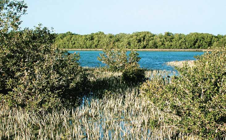
2
INTERTIDAL AND MANGROVE
2.1 INTRODUCTION
Shores of the Red Sea and Gulf of Aden are backed by an
arid zone and in general are fronted by fringing or patch coral
reefs. Rocky shores are usually of raised Quaternary fossil coral
and either form steep undercut cliffs or reef flats cut by wave
action. Inlets (sharms or wadis) occur at intervals formed by
drowned river valleys and provide areas of sheltered soft
sediment forming sand beaches, mudflats with associated salt
marsh and mangrove. Shore temperatures range from a winter
minimum of 8ºC in the northern Red Sea, often with a diurnal
change of 20ºC, to 14ºC in the central Red Sea, but are fully
tropical in the southern Red Sea and Gulf of Aden. Salinities
range from 39­41 ppt at sea, but may rise to hyperhaline
(80­180 ppt) and even hypersaline (80­300 ppt) in coastal
lagoons and intertidal pools. Tides are semi-diurnal and oscillate
around a nodal point near 19ºN with a spring range of 0.6 m in
the north and 0.9 m in the southern Red Sea and 1.5­2.5 m in
the Gulf of Aden.
However there is no appreciable semi-diurnal tide in the
central Red Sea. Strong seasonal changes of up to 0.5 m occur
throughout the Red Sea due to monsoon winds, causing a large
part of the intertidal zone to be inundated during winter months.
These seasonal monsoonal factors must be taken into account
31

---

Standard Survey Methods
when surveying intertidal areas in the central
Methodology for intertidal surveys
region of the Red Sea and exposed regions
recognises the need for measurement of the
such as Socotra, which are subject to periods
physical factors controlling distribution and
of cooler upwelling water.
zonation of biological communities. These
factors were identified in the 1960's for rocky
(LEWIS 1964) and soft sediment shores
The biota of the Red Sea have been
(MCINTYRE 1968) and have been incorporated
studied extensively since the 1700s and in
into texts on survey methodology (HOLME &
general the intertidal biodiversity is now
MCINTYRE 1984; BAKER & WOLFF 1987).
relatively well known (FORSSKAL 1775; JONES
More recently methodology for tropical
et al. 1987; OLIVER 1992; SHEPPARD et al.
biotopes such as mangroves has been
1992; TURNER et al. 1999). There is sufficient
considered (ENGLISH et al. 1997). Adaptation
information to establish regional
of general survey methodology to the region
characteristics (JONES et al. 1987) and to allow
is detailed in BASSON et al. (1977), EDWARDS
comparisons between different biotopes
& HEAD (1987), KRUPP et al. (1996), TURNER
(sand, mud, mangrove, saltmarsh, rock),
et al. (1999) and in numerous research papers
between similar biotopes within the region
(cf. MCCAIN 1984, PRICE & ROBINSON 1993,
and different shore levels within a biotope,
JONES et al. 1998a).
based on presence and absence of species.
These authors identify rapid site
However there is far less information
assessment using key biological species as
available on quantitative aspects of
valuable indicators for distinguishing
abundance, biomass and productivity (JONES
intertidal biotopes. This methodology
et al. 1987; SHEPPARD et al. 1992).
concentrates on recording the presence and
absence of macrobiota (see Appendices 2.6.1
to 2.6.3) and avoids problems of selective
2.2 AIMS OF SURVEYS
collection of small sized (less than 0.5 mm)
organisms. The methodology is relatively
inexpensive and with training does not require
Now that the intertidal biodiversity within
high levels of expertise; in addition the data
the region is known, most surveys are
collected can be used for ground-truthing of
concerned with quantifying the areas of each
satellite imagery and hence used not only on a
biotope within the region. In this way, rarer
local but also at national and regional levels.
biotopes (and their biodiversity) can be
Data should be stored using Geographical
identified and thus protected. Although few, if
Information Systems (GIS) which can be
any, pristine biotopes still exist, the degree of
intercalibrated within the region. Examples of
naturalness and potential for such areas to act
this approach include VOUSDEN (1988),
as replenishment sources also needs to be
KWARTENG & AL-AJMI (1997) and TURNER
established. For conservation objectives it is
et al. (1999).
essential to evaluate the current status of
biodiversity and abundance so that natural
changes can be distinguished from unnatural
For evaluation of long-term fluctuations in
anthropomorphic changes or impacts over
biotopes, either through natural changes or
time and used in integrated environmental
from anthropomorphic impacts, quantitative
assessment (PRICE et al. 1998).
monitoring of permanent transects is
necessary. This approach, which requires
control sites for comparison, has been used
32

---

Intertidal and Mangrove
successfully within the region to evaluate
truthed, all similar biotopes can be classified
intertidal recovery after impact (JONES et al.
throughout the region. For details on
1998a) and to form the basis for monitoring
preparation and usage see KLAUS (1999) and
integrated coastal management plans for the
relevant chapters in this manual. Even if these
Socotra Islands (TURNER et al. 1999).
systems are not used, data should be collected
as indicated below in a form that may be
accessed at a later date for entry into these
Methods for the estimation and
systems.
quantification of marine productivity from
intertidal biotopes are often species specific
and utilise a wide range of biochemical and
2.3.2 Rapid Site Assessment (RSA)
other techniques (IUCN 1987). One of the
most useful is the measurement of natural
This survey method depends upon the
stable carbon and nitrogen isotope ratios
classification of habitats or biotopes by
throughout the food web (RODELLI et al.
recording the presence and absence of key
1984). Although studies have been initiated
species together with a description of the
using this technique for Arabian Gulf
physical characteristics of the habitat.
mudflats (JONES et al. 1998b), they are beyond
Although it is not quantitative the use of key
the scope of the present methodology, which
species presence and absence sheets
concentrates on survey methods for
(Appendices 2.6.1 to 2.6.3) not only enable a
conservation.
biotope to be recognised, but also its range
and overlap with other biotopes to be
ascertained. The survey method is
2.3 SURVEY METHODS
inexpensive, does not require a high level of
training, can be operated with a field team of
two to three persons, and can supply all the
These will vary depending on the survey
information necessary for ground-truthing of
aim and type of intertidal biotope (i.e. soft or
satellite imagery. A further advantage is that
hard substrate). For conservation objectives,
additional sheets (Appendix 2.6.4) can be
these will concentrate on the evaluation of the
designed to record physical descriptions,
current status of biodiversity and abundance
human impact and habitat degradation.
and the distinction between natural and
Examples of the use of these RSA sheets can
unnatural (human-induced) changes over
be found in PRICE (1990), JONES & RICHMOND
time. Scales of survey range from local (e.g.
(1992), JONES et al. (1998a) and TURNER et al.
bay) to national and regional levels and
(1999). Physical data appropriate to each
methodology should allow integration
habitat type are also collected at the same time
between these levels (cf. PRICE et al. 1998).
and used together with the biological data to
classify each biotope (see analysis below).
2.3.1 Remote Sensing and Geographical
Information Systems (GIS)
2.3.3 Species identification
Although initially expensive, these are
The most appropriate and useful
becoming the standard approach to medium
identification guides to biota of the region are
(island) and large-scale (country, region)
given in the section `Identification Guides and
intertidal surveys and allow collection and
Other Recommended Literature' following
transfer of data on a readily accessible basis.
the list of references in section 2.5.
They have the advantage in that, once ground-
33

---

Standard Survey Methods
2.3.4 Quantitative or permanent
calculated. This is achieved by plotting the
monitoring surveys
cumulative number of species against
increasing sample area until no new species
These are used to collect quantitative data
are found (BAKER et al. 1987). Similarity area
on the abundance of intertidal biota over
curves can also be plotted against increases in
extended periods before and after
sample size using Tanimoto Index (presence
anthropomorphic impact (Environmental
and absence of species) and Kulczynski Index
Impact Assessment EIA), to monitor natural
(abundances) to determine optimum sample
environmental changes, or to evaluate
size (see PRENA 1996 for worked examples).
intertidal productivity and links to fisheries.
For a full discussion of comparability and
Methods used are habitat specific and are
reproducibility and more detailed treatment of
given below for each biotope. These surveys
quantitative data see BAKER et al. (1987). At
also require collection of physical data and are
least three replicates should be taken at each
often conducted seasonally. Examples of such
sampling point to allow for calculation of
surveys within the region are given by JONES
variability.
et al. (1987), PRICE et al. (1987), JONES et al.
(1996, 1998a) and TURNER et al. (1999).
2.4 BIOTOPE SPECIFIC
METHODOLOGY
2.3.5 Data analysis
Records of species presence and absence
2.4.1 Sand beaches
from the key species sheets compiled for each
shore visited may be entered onto a computer
These vary greatly both in physical and
database and analysed to determine similarities
biological characteristics, depending upon the
between sites and shore levels. Most useful
degree of exposure to tide and wave action
methods include Hierarchical Agglomeration
ranging from the 100 m plus dune backed
(Cluster Analysis), using, for example,
beaches of Socotra to narrow muddy stretches
Tanimoto Index (PRENA 1996), or diversity
of sand between mangroves and lagoons in
indices such as Shannon-Wiener index
the Red Sea.
(ENGLISH et al. 1997). Principle Component
Analysis can also be used to separate biotopes
or presence and absence of species (PRENA
Physical survey
1996). Physical data can also be analysed,
The exposure index (EI) of MCLACHLAN
using suitable software programmes such as
(1983) is widely used to rank sand beaches.
PRIMER. This can be used to construct cluster
This uses measurement of beach profile, sand
dendrograms, to calculate univariate diversity
grain analysis, organic content, temperature
indices, to measure similarity and dissimilarity
(air and 10 cm below surface), salinity, wave
and to identify the key species responsible for
height, width of swash zone and depth of
dissimilarity, with estimation of their
anoxic black zone, plus presence of
percentage contribution to dissimilarity. For
permanent burrows to determine EI. The
further information, see CLARKE & WARWICK
beach profile between the tide marks is
(1994).
measured using a surveying level and pole
(DALBY 1987) and is related to known tide
levels using local tide tables. Sand grain
For quantitative surveys where abundance
analysis is conducted using sediment samples
data are required, the minimum sample size
of 200 g from the top, mid and bottom of the
needed to estimate diversity must be
beach and, after washing to remove salt,
34

---

Intertidal and Mangrove
analysed by weighing the fractions retained in
Permanent monitoring or quantitative
a series of sieves (BUCHANAN, 1984). Organic
surveys
content is the difference between dry weight
Long-term monitoring sites are usually
of salt free sediment and the weight of this
selected as a result of analysis of RSA surveys
sediment after ashing in a muffle furnace at
to reflect natural biodiversity (control) and
450ºC for 30 minutes. (Dry weight is
sites subject to perturbation. For sand
determined by drying sediment for 24 h at
beaches, permanent transect lines (PTL) are
60ºC). In all cases sediment should be cooled
established from high water spring to low
in a desiccator before weighing to prevent
water spring tides perpendicular to the shore.
uptake of water from the atmosphere. Salinity
Each PTL should be marked with a post set in
may be measured using a refractometer
concrete at the top of the shore and its position
(American Optical Co., USA). Temperature
recorded using GPS. Sampling stations should
and oxygen probes are described in ENGLISH
be positioned at four shore levels: littoral
et al. (1997). Examples of the use of these
fringe (LF), upper eulittoral (UE), lower
measurements to determine EI are given in
eulittoral (LE) and sublittoral fringe (SF).
MCLACHLAN & ERASMUS (1983) and JONES &
These stations are located at tidal levels high
PIERPOINT (1997). The position of each beach
water spring (HWS), high water neaps
should be determined using GPS and Site
(HWN), low water neaps (LWN) and low
Sheets (Appendix 2.6.4) completed on each
water springs (LWS); thus, they will not
beach surveyed.
necessarily be equally spaced, but depend on
the shore profile. This is important as beach
fauna arrange themselves according to tidal
Biological Survey: RSA
level (see JONES 1986).
For RSA, the presence and absence sand
beach key species list (Appendix 2.6.1) may
be used. Observers (two or more) walk on a
Physical data should be collected as
bearing perpendicular to the shore between
outlined in Physical survey above. Epibiota
the tidemarks. All species encountered are
are sampled by taking five random quadrats at
identified and recorded and those difficult to
each station, the quadrat size depending on
identify are labelled and sent to an expert for
species abundance. For example ghost crab
identification. Many sand beach inhabitants
(Ocypode) burrows may require 10 m2
remain buried during low tide so that burrows
quadrats to obtain statistically useful
should be photographed and dug out to
densities, whereas fiddler crab (Uca sp.)
identify burrower and link species to
burrows can be surveyed adequately within
characteristics of burrow. Several of the key
1 m2. Infauna at each station are sampled by
species, such as the amphipod Talorchestia
taking triplicate 25 x 25 x 15 cm deep cores
and isopods Tylos and Eurydice, are relatively
in the sand and sieving, using 1.0 mm mesh.
small (1­5 mm) and may only be revealed by
All material retained should be preserved in
sieving sand through a 1 mm mesh at
5% formalin in seawater for sorting,
intervals down the beach. Once species are
identification and counting in the laboratory.
correctly identified, data from key species
On exposed shores where a large particle size
sheets are entered into the computer and may
is encountered, it may be necessary to first use
be analysed as indicated in 2.3.5.
a 2 mm mesh to remove excess sand. It
should be noted that employment of small
mesh sizes, such as 0.5 mm, would sample
meiofauna, producing abundances of up to
400,000 animals/m2
(MCCAIN
1984);
however macrofaunal biodiversity is
35

---

Standard Survey Methods
sufficient for most conservation surveys. In
be measured 10 cm below the mud surface,
the laboratory each faunal sample is spread
and salinity by placing soil in a syringe with a
out in a shallow tray, just covered with water,
filter paper covering the tip and squeezing
and fauna sorted from residual sediment are
water from the sample onto a refractometer.
identified and counted. Final storage may be
Soil particle size may be measured after the
in 70% alcohol 30% glycerol solution. Rose
removal of gravel and sand by the
Bengal may be used to stain biological
sedimentation technique of BUCHANAN
material to facilitate its separation from sand.
(1984).
For food web surveys it will be necessary
Mudflats are often extensive and can
to use surf plankton nets (COLEMAN &
exceed 1000 m between the tide marks. To
SEAGROVE 1955) and beach seine nets to
mark the profile and sampling levels it is best
sample biota migrating in during high tides.
to time the incoming tide and hence measure
Photography and video filming may be useful
the very shallow profile. While the top levels
to estimate bird populations, and correct
can usually be reached without problems,
completion of site sheets (Appendix 2.6.4)
mud often becomes softer and deeper towards
will ensure anthropomorphic information is
low tide and may best be sampled by boat on
recorded.
a rising tide (MULDER & ARKEL 1980).
2.4.2 Mud flats
Biological Survey: RSA
Methodology is similar to that adopted for
Mud flats are usually found in sheltered
RSAs on sand beaches except that the key
bays, wadis or harbours protected from wave
species sheet (Appendix 2.6.2) should be
action, often in open areas below salt marsh or
used. As most macrofauna of mudflats make
mangrove. They are defined as soft sediment
permanent burrows, time should be spent
shores where the predominant particle size
photographing burrow types and digging out
falls below 64 µm and soil is composed of silt
and identifying occupants so that key species
(3.9­62 µm) and clay (less than 3.9 µm).
can be recognised from burrows. Binoculars
They are often waterlogged and high in
are useful as most species appear on the
organic detritus and subject to microbial
surface at low tide. The presence and extent of
decomposition through oxygen reduction
surface microbial mats should also be
(redox) processes.
recorded. Site sheets (Appendix 2.6.4) should
also be completed. Where the mud is soft it
may be necessary to approach at low tide in a
Physical survey:
small inflatable dingy, moving up the shore on
Measurement of redox potential (Eh) will
the rising tide to survey the shore.
assess the potential impact of additional
organic input as it provides the existing
degree of anoxia (PATRICK & DELAUNE 1977).
Permanent monitoring or quantitative
Eh and pH should be measured onsite by
surveys
digging a hole 20 cm deep into the mud and
Methodology is similar to that for sand
pressing the calibrated platinum electrode of a
beaches where the shore is accessible by foot.
pH/millivoltmeter into the side of the hole
For deep soft mud, grab or core samples must
10 cm from the surface. Readings may be
be taken from a boat operated on the rising
corrected by the addition of +244 mV to give
tide (Fig 2.1). The van Veen grab takes a
Eh (ENGLISH et al. 1997). Temperature should
sample of approximately 0.1 m2 and is the
36

---

Intertidal and Mangrove
lightest of the conventional grabs, as for use in
Saltmarsh occurs throughout the Red Sea,
mud it can be constructed of lightweight
declining towards the more tropical south, and
metals. The corer is made of PVC and
occupies the zone above the mangroves. It is
commonly has a cross-sectional area of
composed of halophytic plants and marks the
0.01 m2 and a length of 1 m. In operation it
landward extension of most marine biota. Due
is thrust or rotated into the sediment to a depth
to high evaporation rates soil salinity may be
of 15 cm with the top end open; a bung is
very high and any fresh water waste run off
then fitted to this end to allow the corer to be
will cause landward extension of marshes.
withdrawn whilst retaining the cored mud.
The halophytes act to stabilise sediment so
The mud is washed through a 1.0 mm mesh
that tidal influences form a network of
sieve hung over the side of the boat and
channels and creeks running between patches
retained biota preserved in 5% formalin in
of vegetation. They are highly productive,
seawater.
shelter abundant bird populations and are of
significance for conservation.
Much of the primary production on
mudflats is carried out by microalgae, a
Physical survey
mixture of pennate diatoms and Cyanophyta
Extensive salt marshes require
known as microbial mats. If these are to be
photographic aerial surveys to map the extent
quantified for food web or other studies it is
of vegetation and channel systems. Profiling
necessary to remove small areas (5 cm2) of
can be conducted using a surveying level and
surface sediment down to 1.5 mm using a
pole but, where marshes are extensive, the use
microscope cover slip. This sediment is made
of the incoming tide to mark height above
up in a known volume of seawater, preserved
chart datum is usually adequate. Collection of
using Lugol's iodine, and cells counted and
data on temperature, salinity, pH, Eh,
identified using a haemocytometer slide.
sediment particle size and organic content is
Alternatively 25 x 25 cm x 0.5 cm deep
similar to that for mudflats (2.4.2).
cores can be taken and chlorophyll extracted
with 90% acetone neutralised with
magnesium carbonate over 24 h, centrifuged
Biological survey: RSA
and the absorption of the supernatant read in a
Methodology is similar to that adopted for
spectrophotometer (details given by BAKER &
RSAs on sand, except that, as for mud shores,
WOLFF 1987).
the key species sheet (Appendix 2.6.2) should
be used. Only the biota listed under the littoral
fringe will be found. However, depending on
As for sand shores tidal immigrants over
freshwater input, a range of up to 20 species
mudflats can be sampled using seine nets,
of saltmarsh plants such as Phragmites and
hadras, or baited traps. Estimation of bird
Typha sp. may occur and reference should be
species and populations can be made by direct
made to HALWAGY et al. (1986), ORME (1982)
observation with binoculars, photography and
and taxonomic descriptions of COLLENETTE
videorecording.
(1985). Site sheets (Appendix 2.6.4) should
be completed.
2.4.3 Saltmarsh
Permanent monitoring or quantitative
Saltmarsh is an area of land bordering the
surveys
sea, more or less covered in vegetation and
Permanent transect lines may be set up
subject to periodic inundation by the tide.
running perpendicular across the marsh and
37

---

Standard Survey Methods
vegetation quantified using 1 m2 quadrats
Biological survey: RSA
(5 replicates) at intervals across the marsh.
Similar methodology applies to that used
Depending on plant size, density (number of
for other soft sediment shores, except for the
plants of each species per quadrat), or cover
use of Appendix 2.6.2 key species sheet using
(area of each species per quadrat when viewed
littoral fringe and upper eulittoral species. All
from above), estimates can be taken to
mangrove species likely to occur within the
quantify species and abundance. However
region are illustrated in RICHMOND (1997). It
care is needed in designing sample strategy if
should be noted that within the region it is
large plants such as Phragmites dominate
likely that species from other key species
(DALBY 1987). Similar 1 m2 quadrats may
sheets (Appendices 2.6.1 to 2.6.3) may occur.
also be used for larger Sesarma or Uca crab
These should be recorded for mixed
burrows and gastropods such as Cerithidea;
communities, including some rocky shore
for smaller infauna, estimates should use the
species settled on mangrove trunks and
25 x 25 x 15 cm deep sediment samples
pneumatophores and sand dwellers, which
sieved through a 1.0 mm mesh (Biological
may coexist (PRICE et al. 1987).
Survey: RSA). Similar methods to those used
for mudflats (2.4.2) can be used to estimate
bird cover.
Permanent monitoring or quantitative
surveys
Methods of quantifying abundance and
2.4.4 Mangroves
biomass of mangrove trees are described in
ENGLISH et al. (1997), but most are not
Although these occur throughout the
applicable to the sparse stands found within
region they are no more than stunted
the region. Where possible, aerial
Avicennia bushes in the northern Red Sea and
photography should be used to determine the
only Avicennia and Rhizophora mucronata are
extent of forest (in many cases this will allow
common in the south, with a total area
tree counts to be made). For much of the Red
regionally of 450­500 km2 (SHEPPARD et al.
Sea region it is possible to measure height and
1992). They grow between HWS and HWN
girth at breast height for trees individually
tide levels and, although usually associated
along a transect vertical to the shore. If stands
with soft mud, may occur on hard bottom
are too abundant for this procedure then the
substrates behind coral reefs on islands. Best
Transect Line Plot method of ENGLISH et al.
development is seen in the southern Red Sea
(1997) is recommended. For other biota, such
where trees reach 5­7 m in height and stands
as microbial mats and macroalgae attached to
may be 100­500 m wide (PRICE et al. 1987).
roots, methods discussed in 2.4.2 and 2.4.5
should be adopted. For macrofauna, 1 m2
quadrat (5 replicates) counts of burrows,
Physical survey
initially identified by digging up their
As the sediments usually consist of soft
inhabitants, will allow quantification;
mud, methods of analysis are those used for
standard 25 x 25 x 15 cm deep sieved
mudflats (2.4.2). Where hard substrate
sediment samples are used for smaller
mangroves exist sediments may be sandier
infauna. Where mud is consolidated or sticky
and methods for sand grain size analysis may
it should be transferred to a bucket of water
apply (2.4.1). Detailed data analysis is given
and broken down gently by hand, before
in ENGLISH et al. (1997), while an example is
sieving through a 1 mm sieve. Smaller
given in AL-KHAYAT & JONES (1999).
quadrats (10 x 10 cm), with five replicates,
can be used to quantify sessile fauna such as
barnacles and mangrove oysters (Saccostrea)
38

---

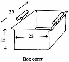
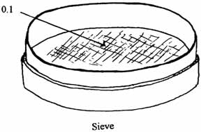
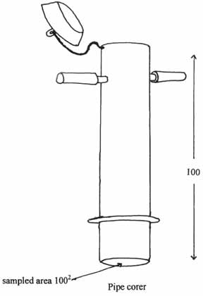
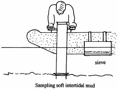
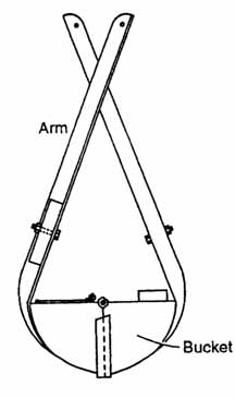
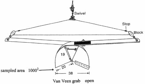
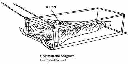
Intertidal and Mangrove
0.1
25
25
15
Sieve
Box corer
sieve
100
Sampling soft intertidal mud
sampled area 1002
Pipe corer
Swivel
Stop
Block
19
Arm
sampled area 10002
20
38
Van Veen grab open
0.1 net
Bucket
Van Veen grab closed
Coleman and Seagrove
Surf plankton net
Figure 2.1 Intertidal sampling gear, all measurements in centimetres
39

---

Standard Survey Methods
attached to trunks and pneumatophores of
discussion on the interaction between physical
mangrove trees. Birds can be estimated by
and biological factors controlling zonation
direct counts, photography and
patterns see JONES et al. (1987).
videorecording. Surveys for mangrove biota,
together with analyses, are presented in AL-
KHAYAT & JONES (1999).
Biological Survey: RSA
Methodology is similar to that used on
soft substrate shores above, except that the
2.4.5 Rocky shores
key species sheet for rocky shores (Appendix
2.6.3) should be used. Strong patterns of
These range from flat terraces extending
vertical zonation are to be expected. There has
out to fringing reefs, often strewn with
been considerable revision of molluscs
boulders, to 1000 m high vertical cliffs on the
recently and BOSCH et al. (1995) and OLIVER
coast of Socotra. The former are described by
(1992) are recommended for gastropod and
FISHELSON (1971) in the northern Red Sea,
bivalve identification respectively. Other taxa
JONES et al. (1987) in the central Red Sea,
can generally be found in RICHMOND (1997).
BARRATT et al. (1987) for the coast of Yemen
Presence of tar and other pollutants covering
and TURNER et al. (1999) for the Socotra
rocks should be noted and recorded on
Islands. A strong pattern of biotic vertical
Appendix 2.6.4 sheets.
zonation is present throughout the region,
although this may be modified seasonally by
changing tide levels in the central Red Sea
Permanent monitoring or quantitative
(JONES et al. 1987) and by cold water
surveys
upwelling on the southern coast of Oman and
Due to the visually obvious nature of
Yemen (BARRATT et al. 1986) and Socotra
rocky shore biota, many methods have been
(TURNER et al. 1999).
devised to measure their abundance and
change over time; for a review see BAKER &
WOLFF (1987). Problems encountered include
Physical survey
the range in size and type of organism (e.g.
Profiles for reef flats may be measured
barnacles and large Sargassum macroalgae),
using a conventional surveying level and pole
topography of the shore, physical danger of
and for vertical cliffs simply using a measuring
wave action on the lower shore and seasonal
tape. However, care must be taken when
changes within the region (see above).
assigning biological zones to tidal heights as
exposure to wave action, shore aspect and
insolation can drastically expand or contract
Once an RSA has been completed, vertical
bands of biotic zonation. Shelter from the sun
biological zones on a shore will have been
under wave-cut notches in cliffs, or under
established. For long-term monitoring a
boulders, will allow lower shore species to
concrete marker can be placed at the top of the
colonise higher positions. Hence it is
shore, and the centre of each biological zone
important to record shade and open shore
marked by drilling a hole in the rock or
surface rock temperatures, together with
hammering in a metal peg. Distances between
temperature and salinity in pools at different
sample sites can be established using a tape
levels on the shore. Lagoons, pools and other
measure. In each biological zone (see
irregularities often trap sediments and these
Appendix 2.6.3) random 1 m2 quadrats can
should be recorded and sampled (see sections
be used (5 replicates) to estimate abundance
2.4.1 and 2.4.2). If measurement of `exposure'
of sessile biota. Flexibility is needed
is required see BAKER & WOLFF (1987). For
depending on the size and abundance of
40

---

Intertidal and Mangrove
individual species, so that barnacles may be
should be used as appropriate to substrate
counted using smaller 10 x 10 cm quadrats,
type. RSA surveys will distinguish the
whereas macroalgae or sponges may require a
differing biological communities and
percentage cover estimate. On exposed shores
appropriate quantitative methods (see above)
many species may shelter under stones, so it
can then be applied.
may be necessary to conduct
counts/percentage cover for the area of the
underside of stones at each level. Providing a
Sabkha, metahaline and hypersaline pools
similar sampling strategy is operated across
These environments are found in flat
the whole shore, data will be valid.
coastal plains, particularly to the north of the
Red Sea, and as they are only intermittently
inundated by the sea are outside the present
Photographic records of permanent
remit. ERLICH & DOR (1985) describe the flora
quadrats are particularly valuable where long-
while POR (1984, 1985) reviews the fauna of
term changes are to be monitored.
these biotopes.
Transparencies taken over time can be
overlaid to visualise changes. Hewlett-
Packard computer plotter and graphics
Artificial structures
programmes are available that use a digitised
These comprise piers, marinas and
pen to count species, provide statistics and
harbours constructed throughout the region.
draw histograms directly from the
In most cases, these simply represent vertical
photographic transparencies.
or sloping rock shores of varying exposure to
wave action and physical and biological
survey methods are appropriate. Where
To assess seasonal succession on rocky
harbours dry at low tide, sands and muds may
shores, areas 1 m2 can be cleared of all biota
be exposed and these may be surveyed using
and monthly estimates of recolonisation
methods detailed for sand and mud shores
made. Similarly, settlement plates (tiles or
above. BASSON et al. (1977) give detailed
slates) secured at different levels on the shore
species lists and zonation patterns for artificial
and removed at intervals will establish
structures.
patterns of colonisation. This approach is
particularly relevant for assessment of
recovery after impact (JONES et al. 1996).
2.4.6 Specialised biotopes
Mixed biotopes
The commonest of these are combinations
of sand, mud and rock coexisting due to shore
topography. Throughout the Red Sea sand
beaches often give way to rock flats towards
low tide. These may have a thin covering of
sand or simply consist of exposed rock.
BASSON et al. (1977) and JONES et al. (1996)
describe these mixed communities in detail.
Methodology described above (2.4.1, 2, 3, 4, 5)
41

---

Standard Survey Methods
2.5 REFERENCES
CLARKE, K.R & WARWICK, R.M. 1994.
Change in marine communities: an approach
to statistical analysis and interpretation.
AL-KHAYAT, J.A. & JONES, D.A. 1999. A
Natural Environment Research Council,
comparison of the macrofauna of natural and
Plymouth Marine Laboratory, Plymouth.
replanted mangroves in Qatar. Estuarine,
Coastal and Shelf Science 49 (Supplement A):
55­63.
COLEMAN, J.S. & SEAGROVE, F. 1955. The
tidal plankton over Stoupe Beck sands, Robin
Hood's Bay (Yorkshire, North Riding).
BAKER, J.M. & WOLFF, M.J. 1987. Biological
Journal Animal Ecology 24: 445­462.
Surveys of Estuaries and Coasts. Cambridge
University Press, Cambridge. 449 pp.
COLLENETTE, S. 1985. An Illustrated Guide to
the Flowers of Saudi Arabia. Scorpion,
BARRATT, L., ORMOND, R.F.E. & WRATHALL,
London. 514 pp.
T. 1986. Ecology and productivity of
sublittoral algae Ecklonia radiata and
Sargassopsis zanardini. Part 1. In: Ecological
DALBY, D.H. 1987. Salt marshes. In:
Studies of Southern Oman Kelp Communities.
Biological Surveys of Estuaries and Coasts.
Council for Conservation of the Environment
(Baker, J.M. & Wolff, W.J. eds): 38­80.
and Water Resources, Muscat, Oman and
Cambridge University Press, Cambridge.
ROPME, Kuwait. 2.1­2. 20 pp.
EDWARDS, A.J. & HEAD, S.M. 1987. Red Sea
BARRATT, L., DAWSON-SHEPPARD, A.R.,
Pergamon Press, Oxford. 441 pp.
ORMOND, R.F.G. & MCDOWALL, R. 1987.
Yemen Arab Republic marine conservation
E
survey. Vol. 1. Distribution of habitats and
NGLISH, S., WILKINSON, C. & BAKER, V.
.
1997. Survey Manual for Tropical Marine
species along the YAR coastline. IUCN Red
Resources 2nd edition. Australian Institute of
Sea and Gulf of Aden Environmental
Marine Science, Townsville. 390 pp.
Programme/TMRU York, UK. 110 pp.
E
B
RLICH, A. & DOR, I. 1985. Photosynthetic
ASSON, P.W., BURCHARD, J.E., HARDY, J.T. &
microorganisms of the Gavish Sabkha. In:
PRICE, A.R.G. 1977. Biotopes of the Western
Hypersaline Ecosystems: The Gavish Sabkha.
Arabian Gulf. ARAMCO, Dhahran. 284 pp.
(Friedman, G.M. & Krumbein, W.E. eds):
296­321. Springer Verlag, Berlin.
BOSCH, D.T., DANCE, S.P., MOOLENBEEK, R.G.
& OLIVER, P.G. 1995. Seashells of Eastern
F
Arabia. Motivate Publishing, London.
ISHELSON, L. 1971. Ecology and distribution
of the benthic fauna in the shallow waters of
296 pp.
the Red Sea. Marine Biology 10: 113­133.
BUCHANAN, J.B. 1984. Sediment Analysis. In:
F
Methods for the Study of Marine Benthos.
ORSSKAL, P. 1775. Descriptiones Animalium
Avium, Amphibiorum, Piscium, Insectorum,
(Holme, N.A. & McIntyre, A.D. eds): 41­65.
Vermium; Quae in Itinere Orientale
Blackwell Scientific Publications, Oxford.
Observavit Petrus Forsskal. Post mortem
auctoris editit Carsten Neibuhr, Copenhagen.
164 pp.
42

---

Intertidal and Mangrove
HALWAGY, R.D., CLAYTON, B. & BEHBEHANI,
JONES, D.A. & PIERPOINT, C.J. 1997. Ecology
M. 1986. Marine Environment and Pollution.
and taxonomy of the Genus Eurydice
In: Proceedings of the First Arabian Gulf.
(Isopoda: Cirolanidae) from sand beaches on
Conference on Environment and Pollution.
the Iberian peninsula. Journal Marine
University of Kuwait, Kuwait. 348 pp.
Biological Association UK 77: 55­76.
HOLME, A. & MCINTYRE, A.D. 1984. Methods
JONES, D.A., PLAZA, J., WATT, I. & AL-SANEI,
for the Study of Marine Benthos 2nd Edition.
M. 1998a. Long-term (1991­1995)
IBP Handbook 16. Blackwell Scientific
monitoring of the intertidal biota of Saudi
Publications, Oxford. 387 pp.
Arabia after the 1991 Gulf War oil spill.
Marine Pollution Bulletin 36: 472­489.
IUCN. 1987. Arabian Gulf. Saudi Arabia: An
Assessment of Biotopes and Coastal Zone
JONES, D.A., AL-ZAIDAN, A. & KENNEDY, H.
Management Requirements for the Arabian
1998b. Role of intertidal mudflats in Gulf
Gulf. MEPA Coastal and Marine Management
ecosystems. Regional Conference on the
Series No. 5. IUCN, Gland.
Marine Environment of the Gulf, University
of Qatar, Doha: 53.
JONES, D.A. 1986. Field Guide to the
Seashores of Kuwait and the Arabian Gulf.
KLAUS, R. 1999. Summary of marine satellite
Blanford Press, Dorset. 192 pp.
image processing and Geographical
Information Systems. In: Conservation and
Sustainable Use of Biodiversity of Socotra
JONES, D.A., GHAMRAWY, M. & WAHBEH, M.I.
Archipelago. Report of Phase 1. (Krupp, F. &
1987. Littoral and shallow subtidal
Hariri, K.I. eds): 9­32. UNOPS YEP/96/G32
environments. In: Key Environments Red Sea.
Contract. C­972248.
(Edwards, A.J. & Head, S.M. eds): 169­193.
Pergamon Press, Oxford.
KRUPP, F., ABUZINADA, A.H. & NADER, I.
1996. A Marine Wildlife Sanctuary for the
JONES, D.A. & RICHMOND, M.D. 1992.
Arabian Gulf. NCWCD, Saudi Arabia.
Intertidal and subtidal marine habitat surveys.
511 pp.
In: Establishment of a Marine Habitat and.
Wildlife Sanctuary for the Gulf Region. Final
Report for Phase 1: 134­160.
KWARTENG, A.Y. & AL-AJMI. 1997. Satellite
Remote Sensing, Applications in the State of.
Kuwait. Kuwait Institute for Scientific
JONES, D.A., WATT, I., PLAZA, J., WOODHOUSE,
Research, Kuwait. 101 pp.
T.D. & AL-SANEI. 1996. Natural recovery of
the intertidal biota within the Jubail Marine
Wildlife Sanctuary after the 1991 Gulf war oil
LEWIS, J.R. 1964. The Ecology of Rocky
spill. In: A Marine Wildlife Sanctuary for the
Shores. English Universities Press Ltd.,
Arabian Gulf. (Krupp, F., Abuzinada, A.H., &
London. 323 pp.
Nader, I.A. eds): 138­158. NCWCD, Saudi
Arabia.
MCCAIN, J.C. 1984. Marine ecology of Saudi
Arabia. The infauna of the sand beaches in the
northern area, Arabian Gulf, Saudi Arabia.
Fauna of Saudi Arabia 6: 53­78.
43

---

Standard Survey Methods
MCINTYRE, A.D. 1968. The meiofauna of
PRENA, J. 1996. The status of the intertidal
some tropical beaches. Journal of Zoology
soft bottom macrofauna six months after the
London 156: 377­392.
Gulf War oil spill. In: A Marine Wildlife
Sanctuary for the Arabian Gulf. (Krupp, F.,
Abuzinada, A.H. & Nader, I.A. eds):
MCLACHLAN, A. 1983. Sandy beach ecology:
128­137. NCWCD, Saudi Arabia.
a review. In: Sandy Beaches as Ecosystems.
(McLachlan, A. & Erasmus, T. eds): 321­380.
Dr. W. Junk, The Hague.
PRICE, A.R.G. 1990. Rapid assessment of
coastal zone management requirements: case
study in the Arabian Gulf. Ocean and.
MCLACHLAN, A. & ERASMUS, T. 1983. Sandy
Shoreline Management 13: 1­19.
Beaches as Ecosystems. Dr. W. Junk, The
Hague.
PRICE, A.R.G., MEDLEY, P.A.H., MCDOWELL,
R.J., DAWSON-SHEPHERD, A.R., HOGARTH, P.J.
MULDER, M. & ARKEL, M.A. 1980. An
& ORMOND, R.F.G. 1987. Aspects of the
improved system for quantitative sampling of
mangal ecology along the Red Sea coast of
benthos in shallow water using the flushing
Saudi Arabia. Journal of Natural History
technique. Netherlands Journal of Sea
21: 449­464.
Research 14: 119­122.
PRICE, A.R.G. & ROBINSON, J.H. 1993. The
OLIVER, P.G. 1992. Bivalved Seashells of the
1991 Gulf War: Coastal and Marine
Red Sea. C. Hemmen, Wiesbaden and Wales.
Environmental Consequences. Marine
330 pp.
Pollution Bulletin 27: 380 pp.
ORME, A.R. 1982. Africa: Coastal Ecology. In:
PRICE, A.R.G., JOBBINS, G., DAWSON-
Encyclopaedia of Beaches and Coastal
SHEPHERD, A.R. & ORMOND, R.F.G. 1998. An
Environments. (Schwartz, M.L. ed.): 3­16.
integrated environmental assessment of the
Hutchinson Ross, Stroudsburg.
Red Sea coast of Saudi Arabia. Environmental
Conservation 25: 65­76.
PATRICK, W.H. & DELAUNE, R.D. 1977.
Chemical and biological redox systems
RICHMOND, M.D. 1997. A Guide to the
affecting nutrient availability in the coastal
Seashores of Eastern Africa. Sida, London.
wetlands. Geoscience and Man 18: 131­137.
448 pp.
POR, F.D. 1984. Notes on the benthic
RODELLI, M.R., GEARING, J.N., GEARING, P.J.,
Copepoda of the mangal ecosystem. In:
MARSHALL, N. & SASEKUMAR, A. 1984. Stable
Hydrobiology of the Mangal (Por, F.D. & Dor,
isotope ratio as a tracer of mangrove carbon in
I. eds): 67­70. Dr. W. Junk Publishers, The
Malaysian ecosystems. Oecologia
Hague.
61: 326­333.
POR, F.D. 1985. Anchialine pools ­
SHEPPARD, C., PRICE, A. & ROBERTS, C. 1992.
comparative hydrobiology. In: Hypersaline
Marine Ecology of the Arabian Region.
Ecosystems (G.M. Friedman & Krumbein
Academic Press, London. 359 pp.
W.E. eds). Ecological Studies 53: 136­144.
44

---

Intertidal and Mangrove
TURNER, J.R., KLAUS, R., SIMOES, N. & JONES,
Salt marsh (see reference list)
D.A. 1999. Littoral and sublittoral ground-
COLLENETTE 1985. An Illustrated Guide to the
truthing survey of the Socotra Archipelago.
Flowers of Saudi Arabia.
In: Conservation and Sustainable Use of.
Biodiversity of Socotra Archipelago. Marine
HALWAGY et al. 1986. Marine Environment
Habitat, Biodiversity and Fisheries Surveys
and Pollution.
and Management. Report of Phase 1.
(Krupp, F. & Hariri, K.I. eds): 33­140.
UNOPS/YEM/96/G32 Contract C­972248.
Sandy beach
JONES, D.A. 1974. The systematics and
VOUSDEN, D.H.P. 1988. The Bahrain Marine
ecology of some sand beach isopods from the
Habitat Survey. Vol. 1. The Technical Report
coasts of Saudi Arabia. Crustaceana 26: 2­11.
ROPME. 103 pp.
VANNINI, M. 1976. Researches on the coast of
Somalia. The shore and dune of Sar Uanle.
Sandy beach decapods. Monitore Zoologico
Identification Guides and Other
Italiano 8: 225­286.
Recommended Literature
VANNINI, M. & VALMORI, P. 1981. Researches
General (see reference list)
on the coast of Somalia. The shore and dune
of Sar Uanle. Monitore Zoologico Italiano 14:
BOSCH
et al. 1995. Seashells of Eastern
199­226.
Arabia.
F
Rocky shore
ISHELSON 1971. Ecology and distribution of
the benthic fauna in the shallow waters of the
DECLERCK, O. & COPPEJANS, E. 1996. Marine
Red Sea.
algae of the Jubail Marine Wildlife Sanctuary,
Saudi Arabia. In: A Marine Wildlife Sanctuary
JONES 1986. Field Guide to the Seashores of.
for the Arabian Gulf. (Krupp, F., Abuzinada,
Kuwait and the Arabian Gulf.
A.H. & Nader, I.A. eds): 199­289. Saudi
Arabia, NCWCD.
JONES et al. 1987. Littoral and shallow
subtidal environments.
HUGHES, R.N. 1977. The biota of reef flats and
limestone cliffs near Jeddah Saudi Arabia.
OLIVER 1992. Bivalved Seashells of the Red.
Journal of Natural History ll: 77­96.
Sea.
G
S
ALIL, B. & VANNINI, M. 1990. Research on
HEPPARD et al. 1992. Marine Ecology of the
the coast of Somalia. Xanthidae, Trapeziidae,
Arabian Region.
Carpiliidae, Menippidae (Crustacea
Brachyura). Tropical Ecology 3: 21­56.
RICHMOND 1997. A Guide to the Seashores of.
Eastern Africa.
POR & DOR 1984. Hydrobiology of the
Mangal.
45

---

Standard Survey Methods
APPENDIX 2.6.1 Key species presence or absence for sandy shores of the Red Sea and Gulf
of Aden.

P/A
R O C A D
LITTORAL FRINGE






Coenobita scaevola






Ocypode saratan






Ocypode cordimana






Tylos exiguus






Talorchestia martensi






UPPER EULITTORAL






Eurydice arabica






Excirolana orientalis






Uca inversa inversa






Uca lactea albimanus






Serenella leachii






Macrophthalmus depressus






LOWER EULITTORAL






Hippa picta






Hippa celaena






Oliva bulbosa






Nassarius clathratus






Macrophthalmus depressus






SUBLITTORAL FRINGE






Echinodiscus auritus






Holothuria arenicola






Calappa hepatica






Thalamita savignyi






Halodule uninervis






Astropecten polycanthus






Thalassodendron ciliatum







P/A, present/absent; R, rare; O, occasional; C, common; A, abundant; D, dominant
46

---

Intertidal and Mangrove
APPENDIX 2.6.2 Key species presence or absence for saltmarsh, mangrove and muddy
shores of the Red Sea and Gulf of Aden.

P/A
R O C A D
LITTORAL FRINGE






Microbial mats (Cyanophyta)






Suaeda monoica






Zygophyllum qartarense






Arthrocnenum macrostachyum






Aeluropus/Juncus






Avicenna marina






Rhizophora mucronata






Uca inversa






Dotilla sulcata






Littorina scabra






Serenella leachii






UPPER EULITTORAL






Uca tetragonon






Uca lactea albimana






Metapograpsus messor






Pirinella conica






Cerithidea cingulata






Periophthalmus koelreuteri






Avicennia marina






Rhizophora mucronata






LOWER EULITTORAL






Potamides conicus






Macrophthalmus depressus






Pinna bicolor






SUBLITTORAL FRINGE






Scylla serrata






Portunus pelagicus






Halophila ovalis






Halodule uninervis








P/A, present/absent; R, rare; O, occasional; C, common; A, abundant; D, dominant
47

---

Standard Survey Methods
APPENDIX 2.6.3 Key species presence or absence for rocky shores of the Red Sea and Gulf
of Aden.

P/A
R O C A D
LITTORAL






Nodolittorina natalensis






Planaxis sulcatus






Acanthopleura vaillantii






Ligia pigmenta






Chthamalus sp.






Chiton peregrinus






Grapsus albolineatus






UPPER EULITTORAL






Nerita undata






Nerita polita orbignyana






Cronia konkanensis






Thais savignyi






Metapograpsus messor/thukuhar






Cellana rota






Balanus amphitrite






Tetraclita squamosa






Enteromorpha sp.






LOWER EULITTORAL






Nerita albicilla






Morula granulata






Laurencia papillosa






Saccostrea cucullata






Ophiocoma scolopendrina






Echinometra mathaei






SUBTIDAL FRINGE






Zoanthus natalensis






Echinometra mathaei






Sargassum sp.






Turbinaria sp.






Colpomenia sinuosa






Corals







P/A, present/absent; R, rare, O, occasional; C, common; A, abundant; D, dominant
48

---

Intertidal and Mangrove
APPENDIX 2.6.4 Site Information.
Latitude
Longitude
Source
Nearest name on map/chart
Sector Code

Researcher
Details of Location
Date Code

21





PROFILE







m


m
1 Mangroves





2 Seagrass





3 Halophytes





FLORA
4 Algae





5 Freshwater
vegetation





6 Other





7
Reefs and corals





8 Birds





9 Turtles





10 Mammals





FAUNA
11 Fish





12 Invertebrates





13 Other





14 Construction





IMPACTS
15
Fishing / Collecting





16 Pollution





17 Other





18 Oceanography





OTHER
19 Meteorology





20 Other





Photographic Record







49

---

Standard Survey Methods
50

---

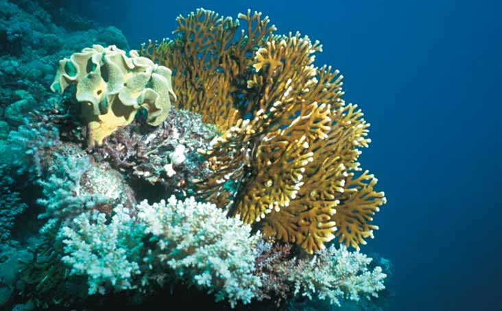
3
CORALS AND CORAL
COMMUNITIES
3.1 INTRODUCTION
Since the 1960s, and in parallel with increasing levels of
human impact, major advances have been made in the survey of
coral reefs (see e.g. STODDART & YONGE 1971; LOYA 1972,
1978; STODDART & JOHANNES 1978; KENCHINGTON 1978; DAHL
1981; DONE 1981, 1982; WEINBERG 1981; DODGE et al. 1982;
ORMOND et al. 1984a; SHEPPARD & SHEPPARD 1985; BROWN
1986; DEVANTIER 1986; HATCHER et al. 1989; ARONSON et al.
1994; ENGLISH et al. 1997; DEVANTIER et al. 1998). These and
many other authors have developed a wide variety of field and
analytical methods for reef surveys, most of which have been
restricted in their application to specific geographical regions or
biogeographic provinces. Although useful in their local areas,
the application of different methods has limited the broadscale
(national, regional or global) comparability of results. This has
meant that the understanding of regional and global trends in the
status of coral reefs has been limited (CONNELL 1997).
The application of different methods in different areas has
also limited the capacity of reef management agencies to
communicate the recent widespread deterioration of reefs to
governments and international conservation agencies (BROWN
1987; WILKINSON 1992; GINSBURG 1994).
51

---

Standard Survey Methods
To facilitate national and regional
REEF RESEARCH IN ARABIA
comparisons, reef survey methods should
follow a standard protocol, as much as is
The RSGA region has a long history of
feasible, given local and national logistic
coral reef research, including some of the
capacities and other constraints. Such
earliest taxonomic work ever undertaken (e.g.
methods should be as simple, quick and
FORSSKAL 1775; EHRENBERG 1834; MILNE
inexpensive as practicable, and be equally
EDWARDS & HAIME 1860). Following these
applicable in nations with different levels of
early studies, and since the beginning of
finance, human capacity and expertise
modern reef studies in the 1960s, the Red Sea
(ARONSON et al. 1994). The application of
(particularly its northern area) has received a
these criteria has culminated in several
great deal of scientific attention (reviews by
regional reef assessment programmes,
MERGNER 1984 and SHEPPARD et al. 1992).
including CARICOMP (OGDEN et al. 1997),
These workers have used a variety of methods
the ASEAN­Australia Living Coastal
to investigate taxonomy, biodiversity, biology,
Resources Project (CHOU & WILKINSON
demography and ecology of corals and other
1992), Reef Check (HODGSON 1999) and the
biota and the environmental properties of the
Global Coral Reef Monitoring Network
ecosystem. By contrast, reefs and coral
(GCRMN, WILKINSON
2000). These
communities of the Gulf of Aden have been
programmes have each produced status
studied less, being largely unknown until
reports that have proven valuable in raising
recently (SHEPPARD et al. 1992; MCCLANAHAN
awareness at both governmental and
& OBURA 1997; KEMP & BENZONI 2000;
intergovernmental levels.
DEVANTIER & HARIRI in press).
In developing a standard protocol of
The following brief review outlines
research methods for coral reefs, the rationale
various methods recently employed in the
and context of the methods should be clear
region, from the broad-scale to the fine-scale.
and the methods prioritised to address key
Broad-scale studies have included habitat
research and management questions. To this
mapping of the central-northern Saudi
end, this chapter briefly reviews reef research
Arabian Red Sea using high definition colour
in the RSGA region, focusing on the study of
aerial photographs (NCWCD­JICA 2000),
corals and coral communities. Rather than
and Socotra Islands Group using LANDSAT
covering the broad field of coral reef studies in
satellite imagery (TURNER et al. 1999). Other
general, this chapter provides an overview of
applications of remote-sensed information
the rationale, advantages and disadvantages of
have included use of broadscale sea surface
various methods for coral reef management-
temperature analyses provided by
related research. Following consultation with
NOAA/NESDIS (GOREAU & HAYES 1994;
national representatives of the PERSGA
GOREAU et al. 1997; STRONG et al. 1997,
expert working-group, the chapter describes a
1998). These images have been used in the
minimum set of methods for site description
interpretation of coral reef bleaching in the
and survey of benthic cover and coral
Saudi Arabian Red Sea, Yemeni Socotra
biodiversity. Recommendations for training,
Islands and Gulf of Aden (DEVANTIER &
quality assurance, data archival, analysis and
HARIRI in press; DEVANTIER et al. in press
presentation, training materials, useful
a,b). All the desk studies relied on extensive
references and a list of relevant world wide
`ground-truthing', generally using rapid
web addresses, are provided.
ecological site assessments (REA).
52

---

Corals and Coral Communities
REA has been used in the RSGA region for
region, have been conducted by SCHEER &
reconnaissance of reef types and condition,
PILLAI (1983), HEAD (1980, 1983), SHEPPARD &
estimates of coral cover and counts of
SHEPPARD (1985, 1991), VERON (1986, 1993,
organisms such as crown-of-thorns starfish,
2000), HOEKSEMA (1989), TURAK & BRODIE
Acanthaster planci, turtles or marine mammals
(1999), WALLACE (1999) and DEVANTIER et al.
(see e.g. ORMOND et al. 1984a­c; MACALISTER
(2000b). Most of these studies have employed
ELLIOT & Partners 1996; WATT 1996; KEMP
variations of a similar field method, i.e. timed
1998; PRICE et al. 1998; TURAK & BRODIE
scuba-swim searches.
1999; DEVANTIER et al. 2000b). Most of these
surveys used semi-quantitative ordinal ranked
categories to describe the habitats, flora and
3.2 METHODOLOGY
fauna, abundances of biological resources,
human uses and impacts. Usually physical
features, shore profiles and environmental
A minimum set of field and analytical
parameters were also recorded.
methods for coral reef research in the Red Sea
and Gulf of Aden are presented below, grouped
under three main headings:
More geographically restricted quantitative
studies using line transects have included
Site description ­ rapid assessment
assessments of coral cover and community
types in Egypt (RIEGL & VELIMIROV 1994;
Benthic cover and abundance of
RIEGL & PILLAR 1999), Saudi Arabia
selected taxa ­ line and belt transects
(ROUPHAEL & AL YAMI 2000; DEVANTIER et al.
(Reef Check, Lifeforms or Video)
2000b) and Yemen (TURAK & BRODIE 1999;
K
Biodiversity assessment (timed scuba-
EMP & BENZONI 2000; DEVANTIER et al. in
press b).
swim searches).
Most of these methods are used widely in
Community composition data have been
the Indo-Pacific, as part of Reef Check and the
recorded at various taxonomic levels, from
GCRMN, and thus provide an additional level
`lifeform' to species. Assessment of recovery
of comparison outside the RSGA region. The
following ship grounding in the Egyptian Red
methods range from simple and inexpensive to
Sea is being undertaken using video transects
the more complex and costly. Although the
and coral settlement plates (S. Clarke, S. Field,
primary purpose of the present chapter is to
pers. comm.). Other applications of video
describe a standard set of coral survey
transects in the Arabian region include the
methods, most of these methods are also
assessment of the effects of the Gulf War and
applied during subsequent monitoring, and
coral bleaching on coral communities of the
thus some of the considerations discussed
Saudi Arabian area of the Arabian Gulf (VOGT
below have relevance to both surveys and
1996; VOGT & AL SHAIKH in press).
monitoring. Prior to conducting a coral reef
survey, several general considerations need to
be addressed.
Considerable taxonomic and biodiversity
research has also been undertaken in the
region. Comprehensive recent studies on
corals, including species from the RSGA
53

---

Standard Survey Methods
3.2.1 Sampling
Stratified sampling designs should
provide information on reef status at various
Design and replication
spatial (local, national and regional) and
A standard survey design for the RSGA
temporal (annual, decadal) scales (Figure
region requires consideration of the spatial
3.1). Within each of the spatial scales,
scales of interest (Figure 3.1). Ideally such
adequate levels of replication are essential for
spatial scales are nested to include:
the statistical description of status and
detection of differences among sites (survey)
Replicate samples within a depth range
and of changes that may occur over time
(monitoring). Ideally, the level of replication
One to several depth ranges within a site
should be based on the results of pilot studies
that identify the major sources and levels of
Replicate sites within a reef
variation, and the likely statistical power of
Reefs within a prescribed area or of a
the sampling design to detect differences
particular type
(ENGLISH et al. 1997; OXLEY 1997; SHEPPARD
1999a).
Areas or reef types within a particular
country
Countries within the region.
Region
Country
Reef type/position across continental shelf
Reef
Zone
Site
Depth
Replicate
Figure 3.1 Example of stratified sampling regime for coral reef monitoring (after ENGLISH et al. 1997,
OXLEY 1997).
54

---

Corals and Coral Communities
For ease of statistical analysis, the
fore reef, back reef) on each reef. Levels of
sampling design should have balanced levels
replication at the reef level depend on the
of replication for:
types of reefs present, whether fringing,
patch, barrier or atoll.
Depths within sites ­ e.g. 3 to 5
transects at one or two depths
3.2.2 Location of Survey Sites
Sites within reefs ­ at least two sites in
each of the different areas (e.g. fore
There are several key criteria that need to
reef, back reef) per reef
be met:
Reefs within reef types ­ e.g. fringing,
Ease of relocation
patch, barrier, atoll.
Sites should be easy to find on the next
survey/monitoring occasion, using maps,
For most of the core methods
navigation charts, landmarks, compass
recommended here, pilot studies have
bearings and portable Global Positioning
determined appropriate levels of within-site
System (GPS) units.
replication:
Reef Check line transects ­ 4 x 20 m
Accessibility
long replicate `segments' (transects) at
Sites should be easily accessible, based on
each of two depths at each site
a realistic assessment of logistic and
(H
budgetary constraints, weather and exposure
ODGSON 1999)
to prevailing sea conditions.
Lifeform line transects ­ 5 x 20 m
long replicate transects at each of two
depths per site (ENGLISH et al. 1997)
Representativeness ­ uniqueness
As much as is practicable given logistic
Reef Check belt transects (abundance
constraints, sites should be representative of
of selected invertebrates and fishes) ­
the different reef types, biotopes and
4 x 100 m2 (5 m wide x 20 m long)
community types present. Similarities and
replicate transects at each of two
variety in habitat and environmental
depths per site, centred on the line
attributes, known histories of the sites
transects (HODGSON 1999)
including effects of disturbance, likely future
Video belt transects ­ 5 x 50 m long
disturbances and any zoning-management
replicate transects at one or two depths
implications in terms of marine protected
per site (OLIVER et al. 1995;
areas (MPAs) all need to be considered in site
SWEATMAN et al. 1998)
selection.
Biodiversity scuba-swim searches ­
3 x 50 minute timed swims at one or
Selection can be aided by initial synoptic
two depths per site.
surveys using manta-tow or similar methods
(ENGLISH et al. 1997). Although not
The level of replication at the site level on
recommended here as a core survey method,
individual reefs is related to reef
manta-tow provides a rapid, inexpensive
geomorphology and exposure and to logistical
means of assessing reef condition, including
constraints. Ideally, at least two sites should
the distribution, extent and status of habitats.
be surveyed in each exposure regime (e.g.
It is a standard field method of REA,
55

---

Standard Survey Methods
employed and recommended by the GCRMN.
recommendations for a depth stratified
The method requires little technical field
sampling design. It is important that samples
support, making it useful for isolated
(replicate transects) within each of these two
locations, and has been employed in many
depth ranges are positioned haphazardly or
reef regions since the 1970s (e.g.
randomly within homogeneous habitats,
KENCHINGTON 1978; OLIVER et al. 1995;
rather than across different habitats.
SWEATMAN et al. 1998).
Recommended depth ranges for biodiversity
surveys of shallow and deep coral
communities depend on local depth-related
Manta-tow requires good field conditions
shifts in community structure, with prior
to be most effective, with water clarity of
surveys in the RSGA region using < 7 m and
more than 10 m, clear skies and low cloud
> 7 m respectively (e.g. DEVANTIER et al.
cover. Trained observers are towed slowly
2000b).
around the reef of interest behind a small
motor boat, at a set speed. Each individual
manta-tow is of set duration (2 min.). The
Where particular site characteristics
boat then stops and the surveyor records a set
preclude the use of the standard depth regimes
of standard observational data onto
(e.g. too shallow, different coral community
waterproof data sheets (e.g. visual estimates
depth distributions or geo-morphological
of coral cover, counts of crown-of-thorns
characteristics etc.), then the precise depth
starfish). The precise geographical position of
range selected is at the discretion of the local
the start and finish of each tow is recorded
survey team. For example, some shallow reefs
using portable GPS, for ease of relocation.
in the RSGA region are less than 7 m in
Manta-tow can be used to select sites for more
depth, with major changes in cover and
detailed quantitative survey, in terms of their
community structure occurring at ca. 3 m
representativeness ­ uniqueness and status.
deep. In such circumstances, shallow sites
should be in the 1­3 m depth range and deep
sites from 4­6 m deep. The depths selected at
Present status
all sites, whether following the standard
Sites should cover the range of different
recommendations or with site-specific
conditions in terms of disturbance, from
alterations, should always be clearly
recently impacted to pristine, rather than
documented on the field data sheets.
concentrating only on reefs in good condition.
This is not to downplay the importance of
surveying sites in excellent or pristine
If two depth ranges are to be surveyed in a
condition. SHEPPARD (1995) provides a useful
single dive, deeper surveys should always be
discussion of the global importance of
conducted first, within conservative dive-time
surveying such sites and of the `shifting base-
limits in accordance with safe diving practice.
line syndrome'.
In particular, great care regarding dive times
should be taken at any sites below 10 m deep,
especially where repetitive diving over
Depth
several days is taking place. Careful
As far as practicable, sites should be
adherence to conservative diving tables and/or
within standard depth ranges. The two
dive computers is mandatory during all diving
standard depth ranges for benthic cover
operations.
surveys are 2­6 m and 7­12 m, consistent
with the Reef Check and GCRMN
56

---

Corals and Coral Communities
3.2.3 Seasonality
tests are available to check for different forms
of bias in the field data (see ENGLISH et al.
As much as is practicable given logistic
1997; OXLEY 1997; DEVANTIER et al. 1999).
constraints, all sites should be surveyed
within a single season, to avoid or minimize
inter-seasonal effects, particularly the rapid
3.2.5 Logistics and Equipment
growth of macroalgae in some reef areas.
National coral reef survey teams will
require the following equipment:
3.2.4 Team Size, Training and Quality
Assurance
Essential
National coral reef survey teams should
Access to reliable land and sea
consist of a minimum of three trained
transport
personnel. This allows for rotation among the
three team members to form a dive team of two
Field camping and cooking equipment
with one person to handle the boat. Larger
Capacity to determine precise field
teams clearly can accomplish more field and
locations ­ maps, navigation charts,
laboratory work, and national teams should be
aerial photographs, compass, portable
expanded as funding and resources permit.
GPS, binoculars
Access to scuba-diving equipment ­
It is most important that all field workers
portable dive compressor, dive tanks,
are consistent in their observations, to
regulators (with spare second-stage
minimize the likelihood of introducing bias in
`octopus', depth-gauge, tank pressure
recording data. OLIVER et al. (1995) identify
gauge, underwater thermometer),
five potential sources of bias, error and
wetsuits, masks, fins, snorkels, dive
imprecision in field data:
knives, dive bags and underwater
carry bags, replacement spares and
Recording ­ transcription
repair kits
Instruments
Waterproof watches
Measurement bias
Safety devices ­ medical kit,
emergency training (e.g.
Sampling bias
resuscitation), dive tables, medical
emergency plan including contact with
Observer bias.
nearest hospital and recompression
chamber, inflatable life-vests, flares,
It is most important that a system of quality
signalling mirror, orange `V sheet',
assurance is developed, to minimize errors in
waterproof torches, water storage
the data collected. This is achieved through
containers
initial training courses in the field methods,
followed with regular refresher courses. Where
Field data sheets and boards
logistics permit, it is highly advantageous to
enter field data directly onto a portable
Tide tables
computer in the field at the end of each day.
Transect tape measures ­ plastic or
This provides the opportunity to check for any
fibreglass for underwater use (3 x
obvious errors immediately. Various statistical
100 m tapes, 10 x 20 m tapes)
57

---

Standard Survey Methods
Geological pick or equivalent hammer
Membership of Diver Alert Network
for collecting coral and other
(DAN) for medical emergency
specimen samples
evacuation.
Sample preservatives and storage bags
3.3 SELECTED METHODS
Computer with spreadsheet and
database programmes.
3.3.1 Site Description
Optional
Various descriptive types of information
4-wheel drive `utility' car for land
are recorded using a rapid assessment method
transport of personnel and equipment
on standard site description data sheets, to aid
the understanding of the present status of the
Seaworthy boat with two motors, oars
site and for ease of relocation in future
and safety equipment for sea transport
surveys. For the survey of coral reefs, these
Diving computers
include:
Underwater stills camera (e.g.
Reef name or other identifier (number
Nikonos V or digital equivalent) with
etc.)
close-up, standard (28 mm and/or 35
mm) and wide-angle (15 mm or 20
Sample identity code (ID) ­ a unique
mm) lenses and strobe flashlight
site descriptor number for each site
that is placed on all data sheets used at
Video camera (digital Hi­8) with
a particular site, linking site
underwater housing and videotapes
description with benthic cover and
10 x 50 m transect tapes for video
biodiversity survey results (see later)
transects
Location ­ GPS position, compass
Portable computer for field data entry
bearings, maps etc.
Steel pegs and heavy hammer for
Survey observers' names
permanently marking transects
Reef type ­ e.g. fringing, patch,
Safety devices ­ portable oxygen-
barrier, atoll
supply kit, radio distress beacon,
Date
hand-held radios or satellite telephone
Reef type
Reef development
Reef slope
Visibility
Exposure to
prevailing wind &
waves
Fringing
1. Extensive (flat > 50 m width)
Average angle
Horizontal
1. Sheltered
Patch
2. Moderate (flat < 50 m width)
to the
using metric
2. Semi-sheltered
horizontal in
tape
Barrier
3. Incipient (no reef flat but some
3. Semi-exposed
increments of
or
accretion)
10 degrees
vertical
Atoll
4. Coral community (coral cover > 10%
using Secchi
4. Exposed
growing directly on non-reefal rock or
disc
sand: and see chapter 5 by Kemp)
Table 3.1 Attributes assessed during site description for coral reefs.
58

---

Corals and Coral Communities
Time of survey
Recommended alpha-numeric site
descriptor codes include the first two alphabet
Tide
initials of each country, followed by a hyphen,
Distance to nearest town
then three numerals for the site number and
then an a or b for deep or shallow depths.
Presence of human litter or rubbish or
Thus, examples for the first site surveyed in
fishing gear above and/or below water
each country are:
Weather conditions ­ approximate
amount of cloud cover, wind speed
Djibouti ­ DJ­001a
Level of reef development (as ranks,
Egypt ­ EG­001a
see later)
Jordan ­ JO­001a
Degree of exposure to waves (as
Saudi Arabia ­ SA­001a
ranks, see later)
Somalia ­ SO­001a
Average angle of reef slope (nearest 10
degrees to horizontal)
Sudan ­ SU­001a
Underwater visibility
Yemen ­ YE­001a
Present status ­ any recent impacts
If two or more teams are working within a
single country, as for example could occur
Type(s) of survey method used: Reef
between the Red Sea, Gulf of Aden and
Check, Lifeform, Video, Biodiversity
Socotra coasts of Yemen, then care must be
Anecdotal information ­ local
taken to allocate unique site codes.
knowledge about the site
Other observations and remarks.
Examples of the ranks used in several of
the site description categories above are
Following the underwater surveys,
provided in Table 3.1. An example of the
additional site description information is
Subtidal Site Description data sheet is
recorded:
provided in Table 3.2 and in Appendix 3.7.1.
Reef Check also provides a standard Site
The presence of any unique or
Description sheet (Appendix 3.7.2), which
outstanding biological features, such
should be completed in addition to the
as particularly large corals or unusual
Subtidal Site Description sheet at all sites
community compositions
where the Reef Check methods are used.
The presence of bleached corals
(partial or total loss of pigments on
Equipment: Maps, navigation charts,
living corals)
aerial photos, tide tables, portable GPS,
compass, binoculars, field data sheets and
The presence of coral predators and
board.
other cause(s) of coral mortality.
59

---

Standard Survey Methods
SITE No:
SU-
Reef Name: Persga Bay Weather:
Fine Date: 15 May 2001 Obs:
001a
Lat:
Depth:
8 ­ 11 Tide:
high
Distance to nearest
m
town: 10 km
Long:
Visibility: Time:
Human
litter:
None
Survey
Reef Check: yes
Lifeform: Video:
Biodiversity:
yes
methods:
Map (show N point and scale)
Profile (show vertical and horizontal distance)

Reef type
Reef development
Other substrata
Exposure
Fring. Patch Barrier Atoll Major Moder- Incip-
Coral



Shelt-
Semi-
Semi-
Expo-
ate
ient
comm.
ered
shelt. expos.
sed
yes




yes

yes
Total
Partial
Slope COT Drup-






Bleaching
Bleaching
angle Stars
ella
yes
20
yes


Notes:
Some partial bleaching, mostly on branching corals, and also low numbers of Drupella snails feeding
on Acropora spp.
Several large massive Porites corals > 3 m in diameter.
No signs of human rubbish or fishing lines, nets etc. No signs of anchor damage.
Table 3.2 Example of partially completed coral reef site description data sheet for a fictitious site in Sudan.
Explanatory Notes:
Site Number ­ identity code, a unique site descriptor number for each site.
Location (latitude, longitude) ­ GPS position, compass bearings, maps, charts etc.
Observers' names, date, time, tide, depth, visibility.
Distance to nearest town ­ approximately, in kilometres.
Visibility ­ note whether the data is from a horizontal underwater measurement (e.g. off transect tape) or a vertical Secchi disc
from the survey vessel; where practicable, always employ the same method.
Human litter ­ rubbish, fishing gear above and/or below water.
Type(s) of survey method used ­ Reef Check, Lifeform, Video, Biodiversity.
Reef type ­ fringing, patch, barrier, atoll.
Reef development ­ major (extensive reef flat > 50 m wide), moderate (reef flat < 50 m wide), incipient reef (some recent
reef accretion but no reef flat), coral community (coral cover > 10% developed directly on non-reef rock, sand or fossil reef).
Other substrata ­ as appropriate.
Exposure to waves ­ sheltered, semi-sheltered, semi-exposed, exposed.
Slope angle ­ (average reef slope angle, nearest 10 degrees to horizontal).
Presence of crown-of-thorns starfish, Drupella snails, total or partial coral bleaching.
Notes ­ anecdotal information, local knowledge about the site, other observations and remarks.
60

---

Corals and Coral Communities
3.3.2 Benthic Cover
Transect number (1­5) can be indicated on the
plastic marker tag by punching the respective
A tiered set of three standard quantitative
number of holes (1­4 for Reef Check, 1­5 for
methods for assessing benthic cover is
Lifeform or Video) through the respective tag.
recommended:
Sub-surface marker buoys or flags are also
appropriate for marking sites, but can have
Reef Check line transects
problems in areas of strong current and/or
wave action, becoming tangled, lost or
Lifeform line transects
collected by fishermen.
Video belt transects
It is particularly important to minimize
This set of methods provides a range of
any damage to the reef during the marking of
options in terms of logistic capacity and
transects, as indeed during all survey work,
expertise, and the amount and detail of data
taking great care not to damage corals and
collected. With increasing expertise, it is
other sessile benthos. This is best achieved by
recommended that national teams progress
good buoyancy control during diving.
from the simplest Reef Check method to the
more complex and data-rich Lifeform and
Video belt methods.
Irrespective of whether survey transects
are marked permanently or not, maps should
be drawn of important conspicuous features of
Positioning and marking of transects
the reefs for ease of site relocation (e.g.
Transects should initially be positioned
position of transects in relation to large
haphazardly or randomly within the chosen
massive corals).
survey habitat, rather than in the best or worst
areas, and should remain within relatively
homogeneous biotopes or community types as
Modifications of the field techniques
far as is practicable. Subsequent to the initial
For ease of statistical comparisons, it is
selection, transects may be fixed permanently
important that the level of replication remains
using steel pegs hammered or cemented into
consistent among sites. In circumstances
the reef substrate. In an initial survey, it is not
where biotopes are small and with little depth
mandatory to mark the precise locations of
profile (e.g. Socotra Islands and Gulf of Aden,
transects with steel stakes and it is at the
Yemen), the standard protocol of positioning
discretion of national teams whether to mark
transects next to each other linearly along the
the precise location of transects.
reef slope may not be appropriate. In such
circumstances, the method should be modified
to ensure that all transects are kept within the
Where transects are to be marked
same biotope with no loss of replication. This
permanently, steel stakes should be placed as
can be achieved by positioning transects
markers in each transect, hammered into the
adjacent to each other but not overlapping (i.e.
substrate every 5 m (for 20 m line transects)
approximately parallel), rather than aligned
or 10 m (for 50 m video transects), with the
linearly along the reef. Sufficient distance
middle stakes smaller than the start and end
should be maintained between adjacent
point stakes. A strong plastic code marker (ca.
transects (e.g. approx. 15 m) to ensure that
8­10 cm long by 4­5 cm wide by 0.2­0.3 cm
transects do not overlap, particularly given
thick) should be attached securely to the first
that fish belt transects (5 m wide) may be
stake of each transect for identification.
centred along the same line transects. Further,
61

---

Standard Survey Methods
and as noted above, where specific site
Equipment: Scuba equipment, data sheets
characteristics do not allow transects to be
and board, transect tape measures (3 x
positioned within the recommended depth
100 m tapes, 3 x 20 m tapes), underwater
ranges (2­6 m and 7­12 m), the survey team
carry-bag, and medical kit.
should select appropriate survey depths.
Data storage: Field data are recorded on
REEF CHECK POINT-INTERCEPT LINE TRANSECTS
waterproof data sheets and input to a
Quantitative assessment of the percentage
spreadsheet (e.g. EXCEL or similar) for storage
cover of 10 categories of sessile benthos is
and preliminary analysis. Examples of the
made using four 20 m line transects, laid
spreadsheets are provided in Appendices 3.7.4
parallel to the selected depth contours at two
and 3.7.7.
depths at each site. The depths surveyed are
7­12 m and 2­6 m below the chart datum of
low water (low tide mark or reef crest where
Where logistics permit, it is advantageous
no chart datum is available). Some sites may
to enter data from the field data sheets directly
not be deep enough to survey both depths.
into the spreadsheet on a portable computer in
the field at the end of each day. This provides
the opportunity to check for any obvious errors
Surveys are conducted by scuba using a
immediately. Subsequently, data may be
100 m long transect tape laid along the
linked into the Reef Check global database.
selected depth contour from a haphazardly or
randomly selected starting point on the reef
slope, with the first 20 m transect starting
Advantages: This method provides a rapid
from the beginning of the tape. The second
means of acquiring quantitative estimates of
transect starts after an interval of 5 m from
percentage cover of the major structural
the end of the first transect (i.e. start at 25 m)
components of coral reefs without requiring
and similarly for the third (start at 50 m) and
detailed taxonomic knowledge, and is thus an
fourth transects (start at 75 m). Deep
ideal first step in developing survey expertise
transects are surveyed first, in accordance
where little capacity exists. The method
with safe diving practice.
requires little in logistic support other than the
essential items listed above.
The 10 categories of benthos (substrate)
recorded in transects are listed in the field data
Disadvantages: The method provides no
sheets (see substrate codes in Table 3.3). On
information on coral community structure and,
each transect, a point sampling method is
because of the limited number of sampling
employed where the substrate located under
points (40 points per 20 m transect), may be
the transect tape at 50 cm intervals is
prone to large variances in heterogeneous
recorded on a waterproof data sheet (Table
habitats. This potential for imprecision can
3.3 and Appendix 3.7.3).
limit the statistical power of the method for
detection of significant trends in cover.
Detailed descriptions and photographs of
the field and analytical methods can be found
Recommendations: This method will
at Reef Check (www.reefcheck.org) and in
form the initial standard survey method for
HODGSON (1999).
coral cover in the RSGA region, being
replaced progressively by more complex
62

---

Corals and Coral Communities
Reef Persga
Site No.
SU-001a








name: Bay
Depth:
15 May
8-11 m Time:
Date:




2001
Team Leader:





Data recorded by:
















Substrate Code













HC hard coral



SC soft coral


DC dead coral

FS fleshy seaweed



SP sponge


RC rock

RB rubble




SD sand


SI silt/clay
OT other






























TRANSECT
1
TRANSECT
2

TRANSECT
3

TRANSECT
4

0 - 19.5 m
25 - 44.5 m
50 - 69.5 m
75 - 94.5 m
0 m
HC
10.0 m
DC
25
m 35
m 50
m 60
m 75
m 85
m
0.5 DC 10.5
OT
25.5 35.5 50.5 60.5 75.5 85.5
1 SD 11.0
HC
26 36 51 61 76 86
1.5 RC 11.5
HC
26.5 36.5 51.5 61.5 76.5 86.5
2 HC 12.0
HC
27 37 52 62 77 87
2.5 OT 12.5
RB
27.5 37.5 52.5 62.5 77.5 87.5
3 RB 13.0
DC
28 38 53 63 78 88
3.5 RB 13.5
DC
28.5 38.5 53.5 63.5 78.5 88.5
4 HC 14.0
HC
29 39 54 64 79 89
4.5 HC 14.5
HC
29.5 39.5 54.5 64.5 79.5 89.5
5 HC 15.0
SD
30 40 55 65 80 90
5.5 FS 15.5
SD
30.5 40.5 55.5 65.5 80.5 90.5
6 FS 16.0
RC
31 41 56 66 81 91
6.5 SC 16.5
FS
31.5 41.5 56.5 66.5 81.5 91.5
7 SP 17.0
FS
32 42 57 67 82 92
7.5 SD 17.5
SP
32.5 42.5 57.5 67.5 82.5 92.5
8 SD 18.0
SP
33 43 58 68 83 93
8.5 SD 18.5
HC
33.5 43.5 58.5 68.5 83.5 93.5
9 SD 19.0
HC
34 44 59 69 84 94
9.5 DC 19.5
HC
34.5 44.5 59.5 69.5 84.5 94.5
Table 3.3 Example of a partially completed Reef Check point-intercept line transect field data sheet at a
fictitious survey site in Sudan.
Explanatory Notes:
Some site description is completed in the top section of the data sheet. A unique site code number is used to link
the transect data with the site description data sheet (see Table 3.2). Results of the point sampling of the four 20
m transects are recorded in the lower portion of the data sheet; for first segment (replicate transect), if the start
point is 0 m, the last point is 19.5 m).
methods as expertise and logistic support
standard method (i.e. 4 x 20 m line transects
develops. The survey design of national
at one or two depths per site), rather than
programmes will depend on capacity and
changing the method. Training can be
logistics, but for ease of statistical comparison
improved by videotaping transects for
within the region, countries with low capacity
subsequent discussion, if logistics permit.
should aim to survey fewer sites using the
63

---

Standard Survey Methods
LIFEFORM LINE-INTERCEPT TRANSECTS
randomly chosen starting positions on the reef
This method provides quantitative
slopes, and may be marked permanently with
estimates of cover of corals and other sessile
steel pegs hammered firmly into the reef
benthic attributes using Lifeform line-
slopes at 5 m intervals.
intercept transects (BRADBURY et al. 1986;
DEVANTIER 1986; ENGLISH et al. 1997). Sets
of five 20 m long transects are surveyed
This method is similar to Reef Check in
using scuba at one or two depths (2­6 m and
that it employs line transects to estimate
7­12 m where appropriate) at the selected
percentage cover of corals and other sessile
survey locations. The transects are laid along
benthic organisms quantitatively. However, it
these depth contours from haphazardly or
differs from Reef Check in that this is a line-
Lifeform
Group Code
Acropora tabular
Scleractinia, Acropora ACT
Acropora branching
Scleractinia, Acropora ACB
Acropora encrusting
Scleractinia, Acropora ACE
Acropora digitate
Scleractinia, Acropora ACD
Acropora submassive
Scleractinia, Acropora ACS
Coral massive
Scleractinia, non-Acropora CM
Coral branching
Scleractinia, non-Acropora CB
Coral submassive
Scleractinia, non-Acropora CS
Coral foliose
Scleractinia, non-Acropora CF
Coral encrusting
Scleractinia, non-Acropora CE
Coral mushroom
Scleractinia, non-Acropora CMR
Heliopora
Alcyonaria, blue coral
CHL
Millepora
Hydrozoa, fire coral
CME
Tubipora musica
Alcyonaria, organ pipe coral
CTU
Soft coral
Alcyonaria, gorgonians, sea whips etc.
SC
Dead coral
Recently dead corals with no visible algae
DC
Dead coral with algae
Dead standing corals with algae
DCA
Sponge Porifera
SP
Zoanthid e.g.
Palythoa, Protopalythoa, Zoanthus spp.
ZO
Other living benthos
Anemones, ascidians etc.
OT
Mixed algal assemblage
Various algae
AA
Coralline Algae
Crustose coralline algae
CA
Turf Algae
Short turf algae
TA
Macro-Algae
Large fleshy algae
MA
Halimeda
Calcareous green algae
HA
Sand
Reefal origin
SD
Rubble
Dead broken coral etc.
RB
Silt Terrestrial
origin
SI
Rock
Rock not covered by other benthos
RCK
Water
Fissures deeper than 50 cm
WA
Other Missing
data
DDD

Table 3.4 Categories of sessile benthic lifeforms surveyed using the GCRMN Lifeform line-intercept
transect protocol (after DEVANTIER 1986; ENGLISH et al. 1997).
64

---

Corals and Coral Communities

SITE No:
SU-001a Reef
Persga Reef Transect
1
Obs:

Name:
No.
Lat:
Depth:
8 ­ 11 m
Tide:
High
Time:
1100 hrs
Date:
15 May
2001
Long:
Visibility: 15 m
Reef type: Fringing
Temp sea: 30 C
Temp air:
33 C





Benthos Transition
Benthos Transition
Benthos Transition
Benthos Transition
Benthos Transition


ACT 105 CF 2000



SD 155



ACB 278



OT 344



CM 389



ACT 490



SD 788



RB 1004



ACB 1466



DCA 1781



RB 1855



CB 1866



CS 1874



DCA 1896



OT 1932



CMR 1938



SD 1965



RB 1977
Table 3.5 Example of data entry for benthic cover on partially-completed Lifeform line-intercept transect
data sheet, for a fictitious survey site in Sudan.
Notes:
General site information is completed in the top section of the data sheet. Results of the line-intercept sampling
of each of five 20 m transects are recorded in the lower portion of the data sheet. The benthic code is recorded
in the left-hand column (under Benthos) and the end-point of that benthic category (= start of the next category
along the transect tape ­ Transition) is recorded (in cm.) in the adjacent right-hand column.
intercept method, rather than point-intercept.
at 50 cm intervals along the transect (Reef
The observer swims slowly along each
Check). Thus the intercept of each sessile
transect, recording the end point (transition)
benthic organism with the transect tape is
of each lifeform (one of the 31 `lifeform'
recorded (Tables 3.4 and 3.5), producing more
categories, Table 3.4) on the standard data
detailed cover data and requiring a more
sheet (Table 3.5 and Appendix 3.7.5), rather
detailed taxonomic knowledge of the benthos
than the benthic attribute located under points
(31 categories instead of 10 as in Reef Check).
65

---

Standard Survey Methods
An example of data entry to the field data
Recommendations: National and regional
sheet is provided in Table 3.5. A detailed
training courses may be initiated once
description of the method is provided in
capacities have developed sufficiently using
ENGLISH et al. (1997).
Reef Check. Regular refresher training
courses may be organized to ensure
consistency in data collection within and
Equipment: scuba equipment, standard
among countries. As with Reef Check,
data sheets and board, transect tape measures
training can be improved by videotaping
(10 x 20 m tapes), underwater carry-bags,
transects for subsequent discussion, where
and medical kit.
logistics permit.
Data storage: Field data are input to the
VIDEO BELT TRANSECTS
ARMDES database provided free of charge
The field methods are similar to line
by the Australian Institute of Marine Science
transects in terms of the positioning of
(AIMS, www.aims.gov.au) for storage and
transects, as described above. Individual video
preliminary analysis of percentage cover. The
transects are longer (50 m) than line transects
data entry programme also provides an error-
(20 m), and a band of benthos is filmed (ca.
checking function. Where logistics permit, it
40 cm wide) rather than a line (DEVANTIER &
is advantageous to enter data from the field
DONE 1995; CHRISTIE et al. 1996; ENGLISH et
data sheets directly onto a portable computer
al. 1997; OXLEY 1997). Series of five replicate
in the field at the end of each day.
transects are filmed at one or two depths per
site, depending on the local reef characteristics
and the discretion of the local survey team.
Advantages: This method requires little
The video operator swims at a constant speed
logistical support and thus is suitable for
(ca. 10­12 m per minute such that a 50 m
isolated locations. Survey observers can be
transect takes 4­5 minutes to film) and height
trained to collect accurate data in a short time
(ca. 25­30 cm) above the transect line. The
period (ca. 1 week training course). The
camera is held perpendicular to the benthos.
method provides data with greater taxonomic
An underwater data sheet showing the site
resolution and usually higher levels of
details, depth and transect number is recorded
precision than does Reef Check. As
prior to filming each video belt transect (Table
observers' levels of taxonomic expertise
3.6). General site characteristics are also
increase, more detailed data can be collected,
filmed. A detailed description of the method is
initially at family-genus level and ultimately
provided in CHRISTIE et al. (1996) and OXLEY
at genus-species level.
(1997).
Disadvantages: The method is more time
Equipment: Scuba equipment, standard
consuming and requires a greater level of
data sheets and board, video camera (digital
taxonomic expertise than Reef Check. For
Hi8), underwater video camera housing and
collection of demographic data, quadrat and
videotapes, ten 50 m transect tape measures.
belt transect methods are more appropriate.
As with other methods, great care must be
taken to ensure all observers are well trained
Data storage: The field data are stored on
and consistent in recording the standard 31
videotapes, with digital archival using
benthic categories (ENGLISH et al. 1997;
compact disc or other digital media.
DEVANTIER et al. 1999).
Quantitative data produced from analysis of
66

---

Corals and Coral Communities
the videotapes are stored in spreadsheets or a
Recommendations: This method should
customized database available from AIMS at
form the third phase in the benthic survey of
www.aims.gov.au.
coral cover in the RSGA region, following
Reef Check point-intercept and Lifeform line-
intercept transects, being phased in as
Advantages: The method is very quick
logistics and capacity allow.
underwater, enabling large numbers of
transects to be recorded in a short period (1 x
50 m transect requires ca. 4 to 5 minutes to
3.3.3 Biodiversity
film) in comparison with Lifeform line-
intercept transects, which can take an
experienced observer more than 30 minutes
Corals
per transect. The method is cost-effective in
terms of laboratory analysis. It also provides a
Scuba swim bio-inventory
permanent videorecord of the survey site,
A detailed inventory of corals is compiled
which is highly useful for showing the
during three replicate timed scuba-swim
characteristics of sites to MPA managers and
searches, each of 50­minutes duration, at one
other decision makers. The results of analysis
or two depths per site. Each of the three
(percentage cover of corals and other sessile
50­minute timed swims is subdivided into
benthos) are compatible with results from line
five 10­minute subsections.
transects, enabling the method to be used as a
follow-up to line transect surveys as expertise
and logistic capacity allow. The video transect
The observers swim slowly along the reef
data are also compatible with more detailed
slope within the chosen depth range,
forms of demographic analysis, by mapping of
recording each coral species seen per
the individual corals present on the transects
10­minute segment onto the standard data
(VOGT 1996).
sheet (Table 3.7 and Appendix 3.7.6). Species
that cannot be readily identified underwater
should be photographed and a sample
Disadvantages: Although cost-effective in
collected for later identification in the
the field and laboratory, the method is reliant
laboratory, where permitted by MPA or other
on expensive equipment, requiring careful
regulations (see below).
maintenance and on-going costs of videotape
archival. The method also requires skilled
personnel for laboratory analysis.
This method provides a comprehensive
coral species list for each site. The method
also provides a crude estimate of relative
Reef
Transect
Persga Bay SITE Code No:
SU-001a
1 Obs:


Name:
No.:
15 May
Temp.
Lat:
Depth:
8 ­ 11m Date:
30 °C
2001
sea:
Long:
Visibility:
15 m
Time:
1200 hrs Tide:
High

Table 3.6 Example of partially completed field data sheet for recording information during filming of video
transects at a fictitious survey site in Sudan. Table is repeated for transects 2 to 5
(see Appendix 3.7.8).
67

---

Standard Survey Methods
abundance of each species at each site, with
Stony ­ hard corals ­ to species wherever
the highest score for any species being 15
possible (VERON & PICHON 1976, 1980, 1982;
(recorded in every 10­minute swim from the
VERON, PICHON & WIJSMAN-BEST 1977;
three replicate 50­minute swim searches).
SCHEER & PILLAI 1983; VERON & WALLACE
With appropriate analysis this method can
1984; VERON 1986, 1993, 2000, 2002;
indicate the types of benthic communities
HOEKSEMA 1989; SHEPPARD & SHEPPARD
present.
1991; SHEPPARD 1997; WALLACE 1999),
otherwise to genus with a description of the
growth form.
Coral taxa are identified underwater to the
following levels, based on the taxonomic
sources cited below:
SITE No: SU-001a Reef Name:
Persga Bay
Date:
15 May 2001
REEF
Lat:
Replicate:
1
Tide: Time:
1200 hrs Obs:

Long:
Visibility:
15 m

Temp sea:
30 C T. air:

Depth: 8 ­ 10 m


Photo:

Field Notes:

































Taxa 0
-
10 - 20 30 40 Taxa 0
-
10 - 20 30 40 Taxa 0
-
10 - 20 30 40
10 20
-
-
-
10 20 -
-
-
10
20
-
-
-
min min 30 40 50
min min 30 40 50
min min 30 40 50
Pdam


Ffung
Lpurp

Pver


Fconc
Ltrans

Shys


Fsimpl

Smam


Fval
E
forsk

Spist


Herpol
E
fruit

Swels


Egem










Mcirc








Mdan








Mmon


Gfasc
Tirreg

Mstil


Easp
Tpel

Mtub


M
elep














Lcory




Aaust


Lhemp

Aclath



Aeuryst


Hexes
Mille

A
form


Hmicr

Agem


Mscher


Table 3.7 Example showing the top half of a coral bio-inventory data sheet, for a fictitious survey site in
Sudan (see Appendix 3.7.6).
Notes:
Some general site information is completed in the top section of the data sheet, with a unique site code number
to link the bio-inventory data to the site description data sheet (Table 3.2). The occurrence of each coral species
in each 10 min. segment of the three 50 min. scuba swims is recorded in the lower portion of the data sheet.
Common coral species in the RSGA region are listed as abbreviations in the left-hand columns. Empty spaces in
the species column are available for the observer to record species not listed in the standard data sheet.
68

---

Corals and Coral Communities
It is recommended that the series of coral
Data storage: Data are stored in
field identification guides `Corals of the
spreadsheets or databases. A typical
World' (VERON 2000) and the CD `Coral ID'
spreadsheet for data storage is easily
(www.aims.gov.au/coralid) be used as the
developed from the field data sheets provided
standard taxonomic reference for stony corals
in Appendices 3.7.6 and 3.7.9.
in the RSGA region. Other useful field
identification aids include HOEKSEMA (1989)
for the family Fungiidae, SHEPPARD &
Advantages:
Semi-quantitative bio-
SHEPPARD (1991), SHEPPARD (1997) for Indian
inventories provide a rapid means of assessing
Ocean corals and WALLACE (1999) for the
biodiversity in comparison with the more
staghorn genus Acropora.
labour-intensive, quantitative quadrat or belt
transect methods. Because of the often-high
numbers of species with low relative
Taxa that cannot be identified reliably to
abundance on coral reefs, quantitative census
species level in the field should be
alone (e.g. quadrats, belt transects, line
photographed (colony and close-up), and a
transects) tends to miss rare species. For this
sample collected for later identification
reason, quantitative assessments are best
(where permitted) using national and/or
combined with semi-quantitative scuba-swim
regional reference collections and in
searches.
consultation with taxonomic experts. Two
comprehensive reference collections exist,
one at NCWCD headquarters (Riyadh) for
Disadvantages: Biodiversity surveys,
stony corals of the central-northern Red Sea
both semi-quantitative and quantitative,
and the other at the Socotra Biodiversity
require a high level of taxonomic expertise
Project headquarters (Hadibo, Socotra) for
and access to reference materials.
stony corals of Socotra, Gulf of Aden and the
Arabian Sea.
Recommendations: Improved taxonomic
capacity should be developed from a series of
Soft corals, gorgonians, zoanthids,
workshops focusing on key taxonomic
anemones and corallimorpharians ­ to genus
groups. Standard reference collections should
or higher taxonomic level, family or order
be assembled in each country and used as
(ALLEN & STEEN 1994; COLIN & ARNESON
often as possible during training courses.
1995; GOSLINGER et al. 1996; REINECKE
1998). Reliable identification to species-level
is presently not possible for many of these
Collecting for Reference
taxa in the field. A comprehensive field guide
Coral samples (specimens) collected for
for the tropical Indo-west Pacific genera of
identification should be small (usually less
soft corals and gorgonians has recently been
than 10 cm on longest axis) and
prepared (FABRICIUS & ALDERSLADE 2000,
representative of the sampled coral colony.
and see www.aims.gov.au for details).
Samples should be carefully removed from
the coral colony in situ, causing minimum
damage, and leaving the remainder of the
Equipment: Scuba equipment, standard
sampled colony intact. For solitary-polyp
data sheets and board, waterproof watch,
mushroom corals, the entire coral is collected.
underwater camera (optional), coral field
All sampling should be kept to the absolute
guides.
minimum necessary for accurate
identification. To achieve this end, surveyors
69

---

Standard Survey Methods
should familiarize themselves with the
cited. A representative selection of the
different species using the taxonomic
bleached, identified coral samples can then be
references cited. For the mushroom corals,
stored as a permanent reference collection.
careful inspection of the ornamentation and
arrangement of septa on the oral (top) and
costae on the aboral surfaces allows field
Other benthos
identification of most species.
Reef Check
The abundance of selected benthic
It is particularly important to take great
organisms is assessed in four belt transects
care when sampling as most corals (and other
20 m long and 5 m wide (100 m2) centred
sessile benthos) are fragile, easily injured and
on the Reef Check line transects (2.5 m either
may become more susceptible to infection and
side of the line) at each site. The organisms
disease. Great care is also required in handling
include: giant clams (Tridacna spp.), pencil
and transporting of specimens to avoid
urchins (Heterocentrotus mammillatus,
breakage, both during the survey and on
Eucidaris spp.), long-spined urchins
return to the laboratory. During transport, all
(Diadema spp.), sea cucumbers (Holothuria
specimens should be carefully wrapped in
scabra, H. fuscogilva, Stichopus chloronotus),
paper and packed securely in a strong, solid
crown-of-thorns starfish (Acanthaster planci),
container, with the heaviest, most robust
giant triton (Tritonia charonis), flamingo
samples (e.g. massive corals) placed at the
tongue (Cyphoma gibbosum), banded coral
bottom, and progressively more delicate
shrimps (Stenopus hispidus) and lobsters
specimens (e.g. stout branching, fine
(Panulirus spp.).
branching, foliose corals) placed on top.
Broken coral (approximate area) and items
While in the field, all specimens should be
of human litter (trash) are also recorded.
labelled with collection information
Photographs of the above species are provided
(specimen code no., site, date, depth, transect
on the Reef Check website.
or replicate no., collector etc.) using a pencil
on a waterproof plastic label tied securely
with fishing line or other suitable material to
The survey observer swims slowly along
the sample. Specimen codes may be the same
each belt transect, searching systematically for
as those used for each site description, with
the organisms listed above, and recording
the addition of a unique specimen number
their occurrence on a standard data sheet
(e.g. spm1, spm2, etc.).
which can be prepared to match the data sheet
in Appendix 3.7.7.
At the base camp or laboratory, the living
coral tissue is removed from the specimens by
Data storage: Data are stored on the
bleaching overnight with household bleach.
standard Reef Check EXCEL spreadsheet
Labels must be securely attached before
(Appendix 3.7.7).
bleaching. Specimens are then soaked and
carefully washed with freshwater and dried.
The dried specimens are examined using a
Advantages: In targeting a small number
hand-lens and/or binocular microscope, and
of easily identified species, the method is
identified, as far as possible, to genus and
quick to learn and easily replicated. These
species level using the taxonomic references
quantitative surveys of selected taxa provide
70

---

Corals and Coral Communities
demographic data not obtainable using the
3.4 DATA ANALYSIS
semi-quantitative methods. A
detailed
description of the method is available on the
There are several key considerations
Reef Check website.
relevant to the efficient storage, analysis and
interpretation of the large amounts of data that
will be produced, in relation to maintaining:
Disadvantages: There is no information
on most non-coral groups, other than the small
Consistency of data types across the
number of target species.
RSGA region
Simplicity and reliability of data entry
Recommendations: Improved taxonomic
systems
capacity should be developed from a series of
workshops focusing on key taxonomic groups.
Reliability of backup and archival
systems
Utility, simplicity and efficiency of
Fish
analytical tools
Detailed guidelines for fish surveys are
provided in a separate chapter of this
Consistency of data presentation and
publication. However, a brief introduction to
reporting.
the Reef Check method is given here.
Consistency of data types should be
Reef Check
maintained by the application of the standard
Four replicate 100 m2 (20 m long x 5 m
methods described herein. For these methods,
wide) belt transects centred on the four 20 m
simple and reliable data entry and archival
line transects (2.5 m either side of the line)
systems have been developed in MICROSOFT
are surveyed in each depth range (7­12 or
EXCEL (i.e. Reef Check and biodiversity data)
2­6 m). Following placement of the transects,
and the ARMDES database (Lifeforms). These
the fish observer should wait for up to
standard methods also have simple and
15 minutes to allow the fishes to resume their
efficient methods of analysis, data presentation
normal behaviour (CARPENTER et al. 1981).
and reporting. For biodiversity surveys, initial
The observer then swims slowly down each
data entry is most simply executed in
transect recording fishes that are distributed
spreadsheets (e.g. EXCEL or equivalent) and
within the borders of the transect on a standard
exported to a custom-designed database (in
data sheet (Appendix 3.7.7). The target fish
ACCESS or equivalent) for long-term storage.
species counted in each transect include:
grouper (Cephalopholis and Epinephelus spp.)
and coral trout (Plectropomus spp.) over
The simplest kinds of analysis are
30 cm in total length (all species), barramundi
descriptive summary statistics, namely mean
cod (Cromileptes altivelis), sweetlips (family
and variance (standard deviation, standard
Haemulidae ­ Plectorhynchus
spp.),
error), mode and median. These are available
humphead (Napoleon/Maori) wrasse
in standard form in most commercial
(Cheilinus undulatus), bumphead parrotfish
spreadsheet and database programmes. A wide
(Bolbometopon muricatum) and butterfly fish
variety of more complex statistical tools is also
(all species of family Chaetodontidae). Details
commercially available for the analysis of
of method and photographs of the fishes are
survey data. These are broadly divisible into
provided at www.reefcheck.org.
univariate and multivariate methods.
71

---

Standard Survey Methods
Univariate analyses are designed to
The application of statistical analysis in
examine differences or trends in one group of
ecology is a complex and rapidly expanding
organisms (e.g. changes in coral cover among
field (e.g. GREEN 1979, 1993; HURLBERT
sites and/or through time, where `repeated
1984; ANDREW & MAPSTONE 1987; JAMES &
measures' type tests (e.g. GREEN 1993) may be
MCCULLOCH
1990; MORRISEY
1993;
appropriate if `fixed' transects are marked
SHEPPARD 1999b). The interested reader is
permanently). These analyses tend to be used
further referred to the references below:
to test null hypotheses of the level of
univariate ­ UNDERWOOD (1981, 1993),
significance of changes or of impacts.
SNEDECOR & COCHRAN (1989), WINER et al.
Univariate analyses are divisible into
(1991), SOKAL & ROHLF (1995); multivariate
parametric and non-parametric tests. For
­ CLIFFORD & STEPHENSON (1975), GRAY et al.
parametric tests, there are several statistical
(1992), CLARKE (1993), JONGMAN et al.
assumptions about the nature of the field data
(1995), DEVANTIER et al. (1998), DE'ATH &
(e.g. normal distribution, homogeneity of
FABRICIUS (2000), DE'ATH (2002).
variances) that need to be met prior to analysis.
The fit of the data to the assumptions can be
examined statistically (e.g. UNDERWOOD
3.4.1 Site Description
1981). For field data that do not meet the
assumptions, various data transformations
Descriptive summary statistics from the
(e.g. square-root transformation, log10 + 1
site description data can be extracted using
transformation, arc-sine transformation etc.)
standard analysis packages in most
are applied to better meet the assumptions, or
spreadsheet programmes. Useful spreadsheet
non-parametric tests (e.g. Kruskal-Wallis
functions include Count and Sum, and the
ANOVA type tests) may be used. For the
summary statistics mean and standard
methods described here, univariate analyses
deviation or standard error, mode and median.
are most useful in examining differences in
In EXCEL, these are found in the `drop-down'
benthic percentage cover (Reef Check point-
menus: Tools ­ Data Analysis ­ Descriptive
intercept transects, Lifeform line-intercept
Statistics.
transects, Video belt transects) and
invertebrate and fish abundances (Reef Check
belt transects).
3.4.2 Benthic Cover
By contrast, multivariate analyses
Reef Check point intercept line transects
examine relationships among multiple groups
To calculate the percentage cover of each
of species (e.g. defining community types) or
of the 10 sessile benthic categories in each
of species with multiple environmental
20 m transect manually, the number of
variables (BROWN 1986; HARGER 1986;
occurrences of each category is summed,
JONGMAN et al. 1995). These analyses tend to
divided by the total possible number of
be used in hypothesis generation, rather than
occurrences (40 points per 20 m transect) and
hypothesis testing. For the methods described
multiplied by 100 to produce a percentage.
here, multivariate analyses are most useful in
Thus, for example, if the sum of occurrences
defining coral community types from the
of hard corals (HC) is 20 points in a transect,
biodiversity data and in exploring
then its percentage cover in that transect is:
relationships among coral communities, coral
20/40 x 100 = 50%.
cover and environmental variables (see later).
72

---

Corals and Coral Communities
This procedure is followed for all of the
The total amount (cover) of coral at
benthic categories present in each transect,
different reefs can vary widely under natural
with the sum of all individual percentage
conditions in relation to differences in
cover calculations equalling 100%.
environment and geomorphology. A useful
interpretation of the results is the
determination of the ratios of live hard coral
To determine the mean or average
to dead coral and total live coral (hard plus
percentage cover of each benthic category at
soft) to dead coral, at each depth and site
one depth (four transects), the percentage
(HODGSON 1999; DEVANTIER et al. 2000b),
cover values for the four transects are added
rather than comparisons of live coral cover
together and divided by four. Thus for
among sites per se.
example, if the four percentage cover values
for hard corals in each of the four transects
are: Transect 1: 50%; Transect 2: 30%;
Lifeform line-intercept transects
Transect 3: 60%; Transect 4: 40%, then the
To calculate the percentage cover of each
mean percentage cover is (50 + 30 + 60 +
of the 31 sessile benthic categories in each
40) divided by 4 = 45%.
20 m transect manually, the total length of the
line-intercept of each category is determined,
then divided by the total length of the transect
Calculations of the mean cover, and the
(20 m) and multiplied by 100 to produce a
level of variation around the mean (standard
percentage. Thus, as a simple example, if the
deviation or standard error), are most easily
intercepts for branching Acropora (ACB) for
performed using standard functions in
Transect 1 (Table 3.8) are:
spreadsheets. In the case of Reef Check, the
field data entry spreadsheet in EXCEL provides
Benthos Transition Intercept
length
calculations of mean percentage cover and
(cm)
variance (standard deviation) at each depth
ACB 50
50
and site (Appendix 3.7.4). Results are usually
CB 100

displayed using bar graphs (see Data
ACB 750
650
SD 1500

Presentation).
ACB 1700
200
DCA 1850

ACB 1950
100
Univariate statistical analysis (usually
SD 2000

analysis of variance ­ ANOVA) is used to

Table 3.8 Example of results of a lifeform line-
examine the significance of differences in
intercept transect, showing benthic categories,
percentage cover between depths at a single
intercepts on the transect (Transition) and the
site, or among sites. The ANOVA model will
calculated length of each lifeform (Intercept length);
vary depending on the particular sampling
benthos symbols from Table 3.4.
design. Suitable software for data analysis is
available in most commercial statistical
then total intercept length for ACB is the
packages. HODGSON (1999) presents regional
sum of the individual intercept lengths: 50 +
and global-scale Reef Check analyses,
650 + 200 + 100 = 1000 cm. Percentage
including multivariate clustering
cover for ACB on this transect is: 1000/2000
dendrograms (Bray-Curtis similarity index)
(total transect length in cm) x 100 = 50%.
and ecological indices of coral reef health and
This procedure is followed for all of the
impact perception.
benthic categories present in each transect,
with the sum of all individual percentage
cover calculations equalling 100%.
73

---

Standard Survey Methods
As with Reef Check, to determine the
Video belt transects
mean or average percentage cover of a benthic
Analysis of a video transect is conducted
category at one depth (five transects), the
initially by point-sampling the videotape on a
percentage cover values for that benthic
television monitor connected to a video editor.
category in the five transects are summed and
Using the video editor, the tape is stopped at
divided by the number of transects (5).
regular intervals (usually 70 stops per 50 m
transect). The identities of the benthos
(usually to genus level for hard and soft
The ARMDES database provided by AIMS
corals) located under five fixed points marked
(www.aims.gov.au) calculates cover and
on the television monitor are recorded into a
abundance (number of intercepts) of each of the
spreadsheet or database for the analysis of
benthic lifeforms recorded per transect, depth
percentage cover (CHRISTIE & MAPSTONE
and site. These results are usually grouped into
1994; CHRISTIE et al. 1996; OXLEY 1997). The
larger summary categories, such as:
five points are marked on the TV screen using
a black permanent marker pen. The points are
Acropora = ACB + ACT + ACE
arranged in a face-centred pattern with two
+ ACS + ACD
points towards the top of the screen, one point
in the centre of the screen and two points
Other hard corals = CB + CS + CMR
towards the bottom of the screen.
+ CM + CE + CF + CME + CHL +
CTU
More detailed demographic data may be
Hard corals = Acropora + other
obtained from the video record by mapping
hard corals
the benthos (VOGT 1996; VOGT et al. 1997),
All live corals = hard corals + soft
rather than by point-sampling. The level of
corals (SC)
taxonomic resolution is dependent on the
expertise of the observer and can be
Dead corals = DC + DCA
standardised by using the same benthic
categories as those of the Reef Check or
Algae = AA + CA + TA + MA + HA
Lifeform transect methods (i.e. the 10 Reef
(Table 3.4).
Check categories, or the 31 Lifeform
categories). For expert observers, video
These summary results are expressed as bar
transects can be analysed at genus and species
graphs of percentage cover (see Data
levels. Once the results are input to a
Presentation). Statistical analysis of differences
spreadsheet or database, typical statistical
among sites is usually conducted with univariate
analyses include ANOVA, although useful
ANOVA type statistics. The ANOVA model will
interpretations can be gained from
vary depending on the particular sampling
multivariate approaches (see section on Data
design. Suitable analysis software is available
Presentation).
on most commercial statistical packages.
As with Reef Check and Lifeform
As with Reef Check, a useful
methods, a useful interpretation of the results
interpretation of the results is the
is the determination of the ratios of live coral
determination of the ratios of live hard coral
to dead coral at each depth and site, rather
to dead coral and total live coral to dead coral
than comparisons of live coral cover among
at each depth and site, rather than comparisons
sites per se.
of live coral cover among sites per se.
74

---

Corals and Coral Communities
3.4.3 Biodiversity
Determine which sites are likely to be
important for replenishment and the
The simplest form of analysis is to
conservation of rare species, important
produce summary descriptive statistics of
in MPA planning (DEVANTIER et al.
species richness at each site, using standard
1998, 2000a,b)
analysis packages provided in most
spreadsheet programmes. Useful spreadsheet
functions include Count and Sum, and the
The coral replenishment index (CI,
summary statistics mean and standard
adapted from DEVANTIER et al. 1998) rates
deviation or standard error, mode and median.
sites based on a combination of their total
In EXCEL for example, these are found in the
coral cover and individual species abundance
`drop-down' menus: Tools ­ Data Analysis ­
scores. Using the present set of methods, the
Descriptive Statistics.
index can be derived from combining the
results of the coral cover transect and the coral
biodiversity surveys for the same site:
The statistical significance of differences
in species richness among sites can be
assessed with ANOVA or similar univariate
CI = AiHi / 100
statistics, using richness values (counts) from
each of the three replicate 50­minute `swim-
where Ai = abundance of the i th hard and
searches' at each site as the base data values.
soft coral taxon at a given depth or site (1­15,
from the bio-inventory surveys) and Hi =
combined percentage cover of hard and soft
Various forms of multivariate analysis
corals at the depth or site (from the benthic
have been used with coral biodiversity data
cover surveys). This index gives highest
(e.g. DONE 1982; SHEPPARD & SHEPPARD
scores to sites that have high species richness,
1991; DEVANTIER et al. 1998, 2000b),
abundance and cover of corals.
principally to define coral community types
and the relations among communities and
various environmental variables. Coral
The Rarity Index (RI, adapted from
community types can be assessed with
DEVANTIER et al. 1998) is derived solely from
various forms of hierarchical cluster analysis,
the biodiversity data. This index rates sites in
using a data matrix composed of species
terms of their species complement of rare
presence ­ absence or relative abundance
versus common coral species:
(1­15) data from all sites. Initially, such
analyses may best be conducted on the
pooled regional data.
RI = Ai / Pi
Additionally, various ecological indices
where Ai = abundance rank for the i th hard
have been used to:
coral taxon at a given site (1­15, from the bio-
inventory surveys) and Pi = the proportion of
Determine which are the key indicator
all sites in which the taxon was present. This
species in different community types
index gives highest values to sites that are
(e.g. D
least representative or most unusual
UFRENE & LEGENDRE 1997;
D
faunistically (i.e. with high abundance of taxa
EVANTIER et al. 2000b)
which are rare in the data set).
Compare sites in terms of the evenness
or dominance of their community
structures (e.g. Shannon-Weaver H')
75

---

Standard Survey Methods
These indices can be calculated in
3.5.2 Benthic Cover
spreadsheets, databases or statistical
packages.
The three recommended methods for
surveying benthic cover (Reef Check line
transects, Lifeform line-intercept transects
A skilled database technician and bio-
and Video belt transects) have a standard
statistician should establish national and
graphical form of presentation, namely bar
regional databases. This proves valuable in
graphs of mean percentage cover and variance
maintaining:
of the important benthic attributes (e.g. hard
corals, soft corals, dead corals, algae etc.). Bar
Consistency of data types across the
graphs are easily produced in all spreadsheet
region
and database programmes. For example, in
EXCEL a variety of different graph types,
Simplicity and reliability of data entry
including bar charts, is available from the
systems
Chart Wizard by following the `drop-down'
menu functions.
Reliability of backup and archival
systems
Utility, simplicity and efficiency of
Reef Check line transects
analytical tools
Preliminary analyses of mean cover and
standard deviation are conducted in the
Consistency of data presentation and
standard Reef Check EXCEL spreadsheet. A
reporting.
typical graphical presentation of mean
percentage cover and variance of hard corals,
dead corals and soft corals derived from Reef
3.5 DATA PRESENTATION
Check line transect data is given in Figure 3.2.
Reporting of survey results should be
standardized as much as is practicable among
Lifeform line-intercept transects
countries within the region. Examples of
Graphical representations of percentage
various reporting formats are provided by
cover results are available within the
OLIVER et al. (1995), SWEATMAN et al. (1998),
ARMDES database. These are typically
Reef Check and GCRMN (WILKINSON 2000).
represented as bar graphs of the mean cover
and variance (standard deviation or standard
error) of the major Lifeform categories at a
3.5.1 Site Description
single site or among different sites.
Site description data should be placed in
the appendices of reports.
Video belt transects
Video transects produce similar results to
Lifeform line transects, that is quantitative
Site locations can be marked on country
estimates of percentage cover of various
maps. Other site description data should be
benthic attributes, usually expressed in bar
placed in a standard table, initially in the data
graphs as mean cover and variance (standard
entry spreadsheet, which may be similar to the
deviation or standard error of the mean,
field data sheets (see Appendices), and
Figure 3.3). Multivariate analyses (e.g.
ultimately exported into a word processing or
various forms of hierarchical clustering,
publishing programme for presentation.
multi-dimensional scaling or principal
76

---

Corals and Coral Communities
70
60
50
40
2
c
o
ver
30
3
6
2
%
5
12
6
23
20
10
0
l
5
6
8
RC1
RC4
RC7
8a
8b
RC1
RC1
RC3
Overa
Site
RC1
RC1
Figure 3.2 Example of results of Reef Check line-transect surveys for percent cover (error bars ­ 1 standard
error) of hard corals (first bar), dead corals (mid bar) and soft corals (third bar) at eight sites in the Saudi Arabian
Red Sea 1998. The numbers above each site show counts of crown-of-thorns starfish (from DEVANTIER et al.
2000b).
acb
acd
aco
acx
2.0
0.8
0.2
0.4
1.0
0.4
0.0
0.0
0.0
0.0
1
2
1
2
1
2
1
2
cb
ce
cf
chl
2.0
2.0
0.8
1.0
1.0
1.0
0.4
0.0
0.0
0.0
0.0
1
2
1
2
1
2
1
2
cm
cmr
cs
ma
2.0
0.8
1.0
0.8
1.0
0.4
0.4
0.0
0.0
0.0
0.0
1
2
1
2
1
2
1
2
s
sc
ta
1.2
2.0
0.8
0.6
0.4
1.0
0.0
0.0
0.0
1
2
1
2
1
2
Figure 3.3 Example of bar graphs illustrating differences in various categories of benthic cover assessed
using sets of five 50 m video belt transects at two sites (1 and 2), with categories: acb ­ Acropora branching,
acd ­ Acropora digitate, aco ­ Acropora corymbose, acx ­ Acropora bottlebrush, cb ­ coral branching, ce ­ coral
encrusting, cf ­ coral foliose, chl ­ coral Heliopora, cm ­ coral massive, cmr ­ coral mushroom, cs ­ coral
submassive, ma ­ macroalgae, s ­ sand, sc ­ soft coral, ta ­ turf algae.
Notes: Typical graphical representation of differences in percentage cover between two monitoring sites. These differences
were significant (1 way ANOVA, alpha 0.05) for Heliopora, coral massive, coral submassive, coral branching and soft corals.
77

---

Standard Survey Methods
components analysis) are also useful means of
­ absence or relative abundance), generated
presenting and interpreting the results
using cluster analysis with various
(e.g. Figure 3.4).
amalgamation schedules and distance
measures. As noted above, there is a multitude
of different statistical approaches to the
3.5.3 Biodiversity
analysis of biodiversity data (see e.g.
JONGMAN et al. 1995 and Figure 3.5).
Typical presentation of biodiversity
results can be as simple as a species ­ site data
matrix table, usually presented as an appendix
It is also useful to combine the analysis of
to the report. More sophisticated presentations
different types of data (site description,
include graphical representations of coral
benthic cover and biodiversity), exploring
community types derived from cluster
relationships among coral community types,
analysis. These can include dendrograms
benthic cover and environmental variables
illustrating the level of similarity among sites
(e.g. Figure 3.6).
based on their species composition (presence
1
acb
acx
sc
acd
cs
s
cf
2
2
1
aco
ma cb
2
2
2
1
cm
1
cmr
1
%
ta
20.26
chl
2
ce
Dim Dim 1 41.05 %
Figure 3.4 Example of principal components analysis biplot of differences in percentage cover of various
lifeform categories in sets of five 50 m video belt transects at two sites (1 and 2). Individual transects are
represented by 1 (Site 1) or 2 (Site 2). acb ­ Acropora branching, aco ­ Acropora corymbose, acd ­ Acropora
digitate, acx ­ Acropora bottlebrush, cf ­ coral foliose, cs ­ coral submassive, cb ­ coral branching, cm ­ coral
massive, cmr ­ coral mushroom, ce ­ coral encrusting, chl ­ coral Heliopora, ma ­ macroalgae, ta ­ turf algae.
Principal component dimensions 1 and 2 account for 61% of the total variance. The vectors (lines) point in the
direction of the highest cover for each of the lifeform categories.
Notes: The biplot is a way of graphically illustrating the relationship among transects in terms of their cover of
the different lifeforms, and clearly indicates differences between the two sites. This analysis and graphical
representation is a useful adjunct to the more commonly applied ANOVA and bar graphs approach.
78

---

Corals and Coral Communities
A
B
C
%
.68
7
2
Dim
D
Dim 1 15.79 %
Figure 3.5 Example of multivariate analysis (hierarchical clustering using Euclidian metric, complete
linkage) showing relationship among sites through species-abundance of four coral community site groups.
Convex hulls delimit four community types A ­ D. Dimensions 1 and 2 account for ~ 24% of the observed
variance. The amount of fill in the bars indicates score of each site on a Rarity Index indicating sites of high
conservation value (data from DEVANTIER et al. 2000b).
ta
A
B
ma
C
D
dc
sc
hc
rbl
%
exp
5
.
5
6
sn
1
dev
2
vis
Dim

Dim 1 71.92 %
ca
Figure 3.6 Example of multivariate analysis (principal components biplot) of relations among cover,
environmental site descriptor variables and coral community types. Dimensions 1 and 2 account for ~ 90%
of the observed variance. The vectors point in the direction of the highest scores for the indicated variables, where
hc ­ stony coral, dc ­ dead coral, sc ­ soft coral, ta ­ turf algae, ca ­ coralline algae, ma ­ macroalgae, sn ­ sand,
rbl ­ rubble, exp ­ exposure, dev ­ reef development, vis ­ water clarity. The symbols represent sites in each of
four coral community type groups A ­ D (data from DEVANTIER et al. 2000b).
79

---

Standard Survey Methods
3.6 REFERENCES
CHRISTIE, C.A. & MAPSTONE, B. 1994. Use of
high resolution video for estimation of
percentage cover of sessile reef benthos.
ALLEN, G.R. & STEEN, R. 1994. Indo-Pacific
Management and Sustainability of Marine
Coral Reef Field Guide. Tropical Reef
Habitats in the 21st Century. Townsville,
Research. 378 pp.
ANZAAS.
ANDREW, N.L. & MAPSTONE, B.D. 1987.
CHRISTIE, C.A., BASS, D.K., NEALE, S.J.,
Sampling and the description of spatial
OSBORNE, K. & OXLEY, W.G. 1996. Surveys of.
pattern in marine ecology. Oceanography and.
sessile benthic communities using the video
Marine Biology Annual Review 25: 39­90.
technique. Standard Operating Procedure No.
2. Australian Institute of Marine Science.
ARONSON, R.B., EDMUNDS, P.J., PRECHT, W.F.,
42 pp.
SWANSON, D.W. & LEVITAN, D.R. 1994. Large
scale, long­term monitoring of Caribbean
CLARKE,
K.R. 1993. Non-parametric
coral reefs: simple, quick, inexpensive
multivariate analyses of changes in
techniques. Atoll Research Bulletin 42: 1­19.
community structure. Australian Journal of.
Ecology 18: 117­143.
BRADBURY, R.H., REICHELT, R.E. & WILLIAMS,
W.T. 1986. Patterns in the structural typology
CLIFFORD, H.T. & STEPHENSON, W. 1975. An
of benthic communities on two coral reefs of
Introduction to Numerical Classification.
the central Great Barrier Reef. Coral Reefs
New York, Academic Press. 229 pp.
4: 161­167.
COLIN, P.L. & ARNESON, C. 1995. Tropical
BROWN, B.E. 1986. Human induced damage
Pacific Invertebrates. California, Coral Reef
to coral reefs. Results of a regional UNESCO
Press. 296 pp.
(COMAR) workshop with advanced training.
UNESCO Reports in Marine Science 40.
CONNELL, J. 1997. Disturbance and recovery
180 pp.
of coral assemblages. Proceedings 8th
International Coral Reef Symposium 1: 9­22.
BROWN, B.E. 1987. Worldwide death of corals
­ natural cyclical events or man­made
DAHL, A.L. 1981. Monitoring coral reefs for
pollution? Marine Pollution Bulletin
urban impact. Bulletin of Marine Science
18: 9­13.
31: 544­551.
CARPENTER, K.E., MICLAT, R.I., ALBALADEJO,
DE'ATH, G. 2002. Multivariate regression
V.D. & CORPUZ, V.T. 1981. The influence of
trees: a new technique for modeling species-
substrate structure on the local abundance and
environment relationships. Ecology 83:
diversity of Philippine reef fishes.
1105-1117.
Proceedings 4th International Coral Reef.
Symposium 2: 497­502.
DE'ATH, G. & FABRICIUS, K. 2000.
Classification and regression trees: a powerful
CHOU, L.M. & WILKINSON, C.R. eds 1992.
yet simple technique for the analysis of
Third ASEAN Science and Technology Week
complex ecological data. Ecology 81:
Conference Proceedings, Marine Science:
3178-3192.
Living Coastal Resources. National
University of Singapore and National Science
and Technology Board, Singapore.
80

---

Corals and Coral Communities
DEVANTIER, L.M. 1986. Studies in the
DEVANTIER, L.M. & HARIRI, K. In press.
assessment of coral reef ecosystems. In:
Coral bleaching in the north-east Gulf of
Human induced damage to coral reefs.
Aden, Summer 1998. In: Proceedings of.
Results of a regional UNESCO (COMAR)
International Workshop on the Extent and
workshop with advanced training (Brown,
Impact of Coral Reef Bleaching in the
B.E. ed). UNESCO Reports in Marine Science
Arabian region. (Abu-Zinada, A. ed). Riyadh,
40: 99­111.
NCWCD.
DEVANTIER, L.M. & DONE, T.J. 1995. Coral
DEVANTIER, L.M., TURAK, E. & AL-SHAIKH,
reef survey and monitoring techniques used at
K. In press a. Coral bleaching in the central-
the Australian Institute of Marine Science. In:
northern Saudi Arabian Red Sea, August-
Proceedings of the Coral Reef Assessment
September 1998. In: Proceedings of.
and Status Evaluation Workshop (Harger,
International Workshop on the Extent and
J.R.E. ed.): 40­50. UNESCO­IOC.
Impact of Coral Reef Bleaching in the
Arabian region. (Abu-Zinada, A. ed). Riyadh,
DEVANTIER, L.M., DE'ATH, G., DONE, T.J. &
NCWCD.
TURAK, E. 1998. Ecological assessment of a
complex natural system: a case-study from the
DEVANTIER, L.M., CHEUNG, C.P.S.,
Great Barrier Reef. Ecological Applications
ABDULAZIZ, M. & KLAUS, R. In press b. Coral
8: 480­496.
bleaching in the Socotra Archipelago, Yemen,
May­June 1998. In: Proceedings of.
DEVANTIER, L.M., SUHARSONO, BUDIYANTO,
International Workshop on the Extent and
A., TUTI, J., IMANTO, P. & LEDESMA, R. 1999.
Impact of Coral Reef Bleaching in the
Status of the coral communities of Pulau
Arabian region. (Abu-Zinada, A. ed). Riyadh,
Seribu, Java Sea, Indonesia. In: Contending
NCWCD.
with Global Change Study No. 10
Proceedings: Coral Reef Evaluation
DODGE, R.E., LOGAN, A. & ANTONIUS, A.
Workshop Pulau Seribu, Jakarta, Indonesia.
1982. Quantitative reef assessment studies in
(Soemodihardjo, S. ed.): 1­24. UNESCO ­
Bermuda: a comparison of methods and
LIPI.
preliminary results. Bulletin of Marine
Science 32: 745­760.
DEVANTIER, L.M., TURAK, E., AL-SHAIKH,
K.A., CHEUNG, C.P.S., ABDUL-AZIZ, M.,
DONE, T.J. 1981. Photogrammetry in coral
DE'ATH, G. & DONE, T.J. 2000a. Ecological
ecology: a technique for studying change in coral
indicators of status of coral communities for
communities. Proceedings 4th International
Marine Protected Areas Planning: Case
Coral Reef Symposium 2: 315­320.
studies from Arabia. In: Information
Management and Decision Support for
DONE, T.J. 1982. Patterns in the distribution of
Marine Biodiversity Protection and Human
coral communities across the central Great
Welfare: Coral Reefs. (Lloyd, D., Done, T.J.
Barrier Reef. Coral Reefs 1: 95­107.
& Diop, S. eds). UNEP, Nairobi.
DUFRENE, M. & LEGENDRE, P. 1997. Species
DEVANTIER, L.M., TURAK, E., AL-SHAIKH,
assemblages and indicator species: The need
K.A. & DE'ATH, G. 2000b. Coral communities
for a flexible asymmetrical approach.
of the central-northern Saudi Arabian Red
Ecological Monographs 67: 345­366.
Sea. Fauna of Arabia 18: 23­66.
81

---

Standard Survey Methods
EHRENBERG, C.G. 1834. Beitrage zur
marine pollution with particular reference to
physiologischen Kenntniss der Corallenthiere
benthos. Rome, FAO Fisheries Technical
im Allgemeinen und besonders des Rothen
Paper 324. 49 pp.
Meeres. Abhandlungen Konigliche Akademie
Wissenschaften Berlin 1832: 250­380.
GREEN, R.H. 1979. Sampling Design and
Statistical Methods for Environmental
ENGLISH, S., WILKINSON, C. & BAKER, V.
Biologists. New York, Wiley. 257 pp.
1997. Survey Manual for Tropical Marine
Resources 2nd Edition. Australian Institute of
GREEN, R.H. 1993. Application of repeated
Marine Science. 390 pp.
measures designs in environmental impact
and monitoring studies. Australian Journal of.
FABRICIUS, K. & ALDERSLADE, P. 2000. Soft
Ecology 18: 81­98.
Corals and Sea Fans: A comprehensive guide
to the tropical shallow-water genera of the
HARGER, J.R.E. 1986. Responses of coral reef
central west Pacific, the Indian Ocean and the
communities to environmental variables in the
Red Sea. Australian Institute of Marine
Kepuluaun Seribu Island chain. In: Human
Science. 272 pp.
induced damage to coral reefs. Results of a
regional UNESCO (COMAR) workshop with
FORSSKAL, P. 1775. Descriptiones Animalium
advanced training. (Brown, B.E. ed).
Avium, Amphibiorum, Piscium, Insectorum,
UNESCO Reports in Marine Science
Vermium; Quae in Itinere Orientale
40: 164­173.
Observavit Petrus Forsskal. Post mortem
auctoris editit Carsten Neibuhr, Copenhagen.
HATCHER, B.G., JOHANNES, R.E. &
164 pp.
ROBERTSON, A.I. 1989. Review of research
relevant to the conservation of shallow
GINSBURG, R. (Compiler) 1994. Proceedings
tropical marine ecosystems. Oceanography
of the colloquium on global aspects of coral
and Marine Biology Annual Review:
reefs: health, hazards and history. Miami,
27: 337­414.
Rosenstiel School of Marine and Atmospheric
Science, University of Miami. 420 pp.
HEAD, S.M. 1980. The ecology of corals in the
Sudanese Red Sea. PhD Thesis, University of
GOREAU, T.J. & HAYES, R.L. 1994. Coral
Cambridge.
bleaching and ocean hotspots. Ambio
23: 176­180.
HEAD, S.M. 1983. An undescribed species of
Merulina and a new genus and species of
GOREAU, T.J., HAYES, R.L. & STRONG, A.E.
siderastreid coral from the Red Sea. Journal
1997. Tracking south Pacific coral reef
of Natural History 17: 419­435.
bleaching by satellite and field observations.
Proceedings 8th International Coral Reef.
HODGSON, G. 1999. A global assessment of
Symposium 2: 1491­1494.
human effects on coral reefs. Marine
Pollution Bulletin 38: 345­355.
GOSLINGER, T.M., BEHRENS, D.W. &
WILLIAMS, G.C. 1996. Coral Reef Animals of.
HOEKSEMA, B.W. 1989. Taxonomy, phylogeny
the Indo-Pacific. Monterey, USA, Sea
and biogeography of mushroom corals
Challengers.
(Scleractinia: Fungiidae). Zoologische
Verhandelingen 254: 1­295.
GRAY, J.S., MCINTYRE, A.D. & STIRN, J. 1992.
Manual of Methods in Aquatic Environment
Research. Part II ­ Biological assessment of.
82

---

Corals and Coral Communities
HURLBERT, S.H. 1984. Pseudoreplication and
MCCLANAHAN, T.R. & OBURA, D. 1997.
the design of ecological field experiments.
Preliminary ecological assessment of the Saad
Ecological Monographs 54: 187­211.
ed Din, Awdal region. Somali Natural
Resources Management Programme. IUCN
JAMES, F.C. & MCCULLOCH, C.E. 1990.
Eastern African Programme. 45 pp.
Multivariate analyses in ecology and
systematics: Panacea or Pandora's box?
MERGNER, H. 1984. The ecological research
Annual Review of Ecology and Systematics
on coral reefs of the Red Sea. Deep Sea
21: 129­166.
Research A 31: 855­884.
JONGMAN, R.H.G., TER BRAAK, C.J.F. & VAN
MILNE EDWARDS, H. & HAIME, J. 1860.
TONGEREN, O.F.R. 1995. Data analysis in
Histoire Naturelle des Coralliaires. 3 Vols.
community and landscape ecology.
Paris. pp. 1­560.
Cambridge University Press. 299 pp.
MORRISEY, D.J. 1993. Environmental Impact
KEMP, J. 1998. The zoogeography of the coral
Assessment ­ a review of its aims and recent
reef fishes of the Socotra Archipelago.
developments. Marine Pollution Bulletin 26:
Journal of Biogeography 25: 919­933.
540­545.
KEMP, J.M. & BENZONI, F. 2000. A
NCWCD­JICA 2000. Final report of the study
preliminary study of coral communities in the
on coastal/marine habitats and biological
northern Gulf of Aden. Fauna of Arabia
inventories in the northern part of the Red Sea
18: 67­86.
coast in the Kingdom of Saudi Arabia.
Unpublished report to NCWCD, Riyadh.
KENCHINGTON, R.A. 1978. Visual surveys of
large areas of coral reefs. In: Coral Reefs:
OGDEN, J. & 32 OTHERS. 1997. Caribbean
Research Methods. (Stoddart, D.R. &
coastal marine productivity (CARICOMP): A
Johannes, R.F. eds): 149­161. UNESCO, Paris.
research and monitoring network of marine
laboratories, parks and reserves. Proceedings
LOYA, Y. 1972. Community structure and
8th International Coral Reef Symposium
species diversity of hermatypic corals at Eilat,
1: 641­646.
Red Sea. Marine Biology 13: 100­123.
OLIVER, J., DE'ATH, G., DONE, T., WILLIAMS,
LOYA, Y. 1978. Plotless and transect methods.
D., FURNAS, M. & MORAN, P. 1995. Long-term
In: Coral Reefs: Research Methods. (Stoddart,
monitoring of the Great Barrier Reef Status
D.R. & Johannes, R.F. eds.): 197­217.
Report Number 1. Australian Institute of
UNESCO, Paris.
Marine Science. 121 pp.
MACALISTER ELLIOTT AND PARTNERS LTD.
ORMOND, R.F.G., DAWSON-SHEPHERD, A.,
1996. Mission Report (Marine Team).
PRICE, A. & PITTS, R.G. 1984a. Report on the
Biodiversity Conservation and Sustainable
distribution of habitats and species in the Saudi
Development Programme. Socotra
Arabian Red Sea. IUCN/MEPA/PERSGA,
Archipelago, Republic of Yemen. UNDP,
Jeddah, Kingdom of Saudi Arabia. 123 pp.
GEF, and MacAlister Elliott & Partners,
Lymington, Hampshire. 42 pp.
ORMOND, R.F.G., DAWSON-SHEPHERD, A.,
PRICE, A. & PITTS, R.G. 1984b. Report on the
distribution of habitats and species in the Saudi
Arabian Red Sea. 2. IUCN/MEPA/PERSGA,
Jeddah, Kingdom of Saudi Arabia. 151 pp.
83

---

Standard Survey Methods
ORMOND, R.F.G., DAWSON-SHEPHERD, A.,
SHEPPARD, C.R.C. 1997. Indian Ocean Marine
PRICE, A. & PITTS, R.G. 1984c. Management
Life Guides Corals of the Indian Ocean.
of Red Sea coastal resources:
Compact Disc produced by SIDA Regional
recommendations for protected areas.
Coral Reef Programme, Stockholm
IUCN/MEPA/PERSGA, Jeddah, Kingdom of
University, Sweden, and the Dept. of
Saudi Arabia. 113 pp.
Biological Sciences, University of Warwick,
United Kingdom.
OXLEY, W.G. 1997. Sampling design and
monitoring. In: Survey Manual for Tropical
SHEPPARD, C.R.C. 1999a. Coral decline and
Marine Resources 2nd Edition. (English, S.,
weather patterns over 20 years in the Chagos
Wilkinson, C. & Baker, V. eds): 307­320.
Archipelago, Central Indian Ocean. Ambio
Australian Institute of Marine Science.
28: 472­478.
PRICE, A.R.G., JOBBINS, G., DAWSON
SHEPPARD, C.R.C. 1999b. How large should
SHEPHERD, A.R. & ORMOND, R.F.G. 1998. An
my sample be? Some quick guides to sample
integrated environmental assessment of the
size and the power of tests. Marine Pollution
Red Sea coast of Saudi Arabia. Environmental
Bulletin 38: 439­447.
Conservation 25: 65­76.
SHEPPARD, C.R.C. & SHEPPARD, A.L.S. 1985.
REINICKE, G.B. 1998. Xeniidae (Coelenterata:
Reefs and coral assemblages of Saudi Arabia
Octocorallia) of the Red Sea, with
1. The central Red Sea at Yanbu al Sinaiyah.
descriptions of six new species of Xenia.
Fauna of Saudi Arabia 7: 17­36.
Fauna of Saudi Arabia 16: 5­62.
SHEPPARD, C.R.C. & SHEPPARD, A.L.S. 1991.
RIEGL, B. & PILLER, W.E. 1999. Coral
Corals and coral communities of Arabia.
frameworks revisited-reefs and coral carpets
Fauna of Saudi Arabia 12: 3­170.
in the northern Red Sea. Coral Reefs
18: 241­253.
SHEPPARD, C.R.C., PRICE, A. & ROBERTS, C.
1992. Marine Ecology of the Arabian Region
RIEGL, B. & VELIMIROV, B. 1994. The
­ Patterns and Processes in Extreme Tropical
structure of coral communities at Hurghada in
Environments. Academic Press, London.
the northern Red Sea. PSZN Marine Ecology
345 pp.
15: 213­231.
SNEDECOR, G.W. & COCHRAN, W.G. 1989.
ROUPHAEL, T. & AL YAMI, H. 2000. Wide-
Statistical Methods 8th Edition. Iowa State
scale survey of live and dead coral, crown-of-
University Press, Iowa. 503 pp.
thorns starfish (Acanthaster planci) and the
gastropod Drupella in the Farasan Islands
SOKAL, R.R. & ROHLF, F.J. 1995. Biometry.
Marine Protected Area. Technical report to
The Principles and Practice of Statistics in
NCWCD, Riyadh. 31 pp.
Biological Research. 3rd Edition. W.H.
Freeman & Co., San Francisco. 850 pp.
SCHEER, G. & PILLAI, C.S.G. 1983. Report on
the hard corals from the Red Sea. Zoologica
STODDART, D.R. & YONGE, M. (eds) 1971.
45 (133): 198 pp.
Regional Variation in Indian Ocean Coral
Reefs. Symposium of the Zoological Society
SHEPPARD, C.R.C. 1995. The shifting base-
of London 28.
line syndrome. Marine Pollution Bulletin
30: 766­767.
84

---

Corals and Coral Communities
STODDART, D.R. & JOHANNES, R. 1978. Coral
VERON, J.E.N. 1986. Corals of Australia and.
Reefs: Research Methods. UNESCO, Paris.
the Indo-Pacific. Angus and Robertson,
581 pp.
Australia. 644 pp.
STRONG, A.E., BARRIENTOS, C.S., DUDA, C. &
VERON, J.E.N. 1993. A Biogeographic
SAPPER, J. 1997. Improved satellite techniques
Database of Hermatypic Corals Species of the
for monitoring coral reef bleaching.
Central Indo-Pacific Genera of the World.
Proceedings 8th International Coral Reef.
Australian Institute of Marine Science
Symposium 2: 1495­1498.
Monograph Series Vol. 10. 433 pp.
STRONG, A.E., GOREAU, T.J. & HAYES, R.L.
VERON, J.E.N. 2000. Corals of the World. 3
1998. Ocean hotspots and coral reef
Vols. Australian Institute of Marine Science.
bleaching. January­July 1998. Reef.
Encounter 24: 20­22.
VERON, J.E.N. 2002. New Species Described.
in Corals of the World. Australian Institute of
SWEATMAN, H., BASS, D., CHEAL, A.,
Marine Science Monograph Series, Vol. 11.
COLEMAN, G., MILLER, I., NINIO, R., OSBORNE,
209 pp.
K., OXLEY, W., RYAN, D., THOMPSON, A. &
TOMKINS, P. 1998. Long-term monitoring of the
VERON, J.E.N. & PICHON, M. 1976.
Great Barrier Reef Status Report Number 3.
Scleractinia of Eastern Australia. Part I
Australian Institute of Marine Science. 303 pp.
Families Thamnasteriidae, Astrocoeniidae,
Pocilloporidae. Australian National
TURAK, E. & BRODIE, J. 1999. Coral and reef
University Press, Canberra, Australian
habitats. In: Ecosystems of the Red Sea Coast
Institute of Marine Science Monograph
of Yemen. Protection of Marine Ecosystems of.
Series 1. 86 pp.
the Red Sea Coast of Yemen. (DouAbul, A.,
Rouphael, T. & Marchant, R. eds): 17­39.
VERON, J.E.N. & PICHON, M. 1980.
Hassell & Assoc., AMSAT and UNOPS.
Scleractinia of Eastern Australia. Part III
Families Agariciidae, Siderastreidae,
TURNER, J., KLAUS, R., SIMOES, N. & JONES,
Fungiidae, Oculinidae, Merulinidae,
D.A. 1999. Littoral and sublittoral ground-
Mussidae, Pectiniidae, Caryophylliidae,
truthing survey of the Socotra Archipelago.
Dendrophylliidae. Australian National
In: Conservation and Sustainable Use of.
University Press, Canberra, Australian
Biodiversity of Socotra Archipelago. Marine
Institute of Marine Science Monograph
Habitat, Biodiversity and Fisheries Surveys
Series 4. 422 pp.
and Management. Report of Phase I. (Krupp,
F. & Hariri, K.I. eds): 33­139. Senckenberg
VERON, J.E.N. & PICHON, M. 1982.
Research Institute, Frankfurt a.M., Germany.
Scleractinia of Eastern Australia. Part IV.
Family Poritidae. Australian National
UNDERWOOD, A.J. 1981. Techniques of
University Press, Canberra, Australian
analysis of variance in experimental marine
Institute of Marine Science Monograph
biology and ecology. Oceanography and
Series 5. 159 pp.
Marine Biology Annual Review 19: 513­615.
VERON, J.E.N., PICHON, M. & WIJSMAN-BEST,
UNDERWOOD, A.J. 1993. The mechanics of
M. 1977. Scleractinia of Eastern Australia.
spatially replicated sampling programmes to
Part II. Families Faviidae, Trachyphylliidae.
detect environmental impacts in a variable
Australian National University Press,
world. Australian Journal of Ecology
Canberra, Australian Institute of Marine
18: 99­116.
Science Monograph Series 1. 233 pp.
85

---

Standard Survey Methods
VERON, J.E.N. & WALLACE, C.C. 1984.
WILKINSON, C.R. 1992. Coral reefs of the
Scleractinia of Eastern Australia. Part V.
world are facing widespread devastation: can
Family Acroporidae. Australian National
we prevent this through sustainable
University Press, Canberra, Australian
management practices? Proceedings 7th
Institute of Marine Science Monograph
International Coral Reef Symposium 1:
Series 1. 485 pp.
11­21.
VOGT, H. 1996. Investigations on coral reefs
WILKINSON, C.R. 2000. Status of Coral Reefs
in the Jubail Marine Wildlife Sanctuary using
of the World: 2000. Global Coral Reef
underwater video recordings and digital
Monitoring Network and Australian Institute
image analysis: In: A Marine Wildlife
of Marine Science. 363 pp.
Sanctuary for the Arabian Gulf.
Environmental Research and Conservation
WINER, B.J., BROWN, D.R. & MICHELS, K.M.
Following the 1991 Gulf War Oil Spill.
1991. Statistical Principles in Experimental
(Krupp, F., Abuzinada, A.H. & Nader, I.A.
Design. 3rd edition. McGraw-Hill, New York.
eds): 302­326. Forschungsinstitut
1057 pp.
Senckenberg, Frankfurt & NCWCD, Riyadh.
Other Recommended Literature
VOGT, H., MONTEBON, A.R.F. & ALCALA,
M.L.R. 1997. Underwater video sampling: an
ABUZINADA, A. ed. In press. Proceedings of.
effective method for coral reef surveys?
the International Workshop on the Extent and.
Proceedings 8th International Coral Reef.
Impact of Coral Bleaching in the Arabian
Symposium 2: 1447­1452.
region. NCWCD, Riyadh.
VOGT, H.P. & AL-SHAIKH, K. in press. Status
ANTONIUS, A., SCHEER, G., & BOUCHON, C.
of Saudi Arabian coral reefs in the Arabian
1990. Corals of the Eastern Red Sea. Atoll
Gulf following coral bleaching in 1997/1998.
Research Bulletin 334: 1­22.
In: Proceedings of International Workshop on
the Extent and Impact of Coral Reef.
AVISE, J.C. 1994. Molecular Markers, Natural
Bleaching in the Arabian region. (Abu-
History and Evolution. Chapman and Hall,
Zinada, A. ed). Riyadh, NCWCD.
USA. 511 pp.
WALLACE, C.C. 1999. Staghorn corals of the
BEHAIRY, A.K.A., SHEPPARD, C.R.C. & EL-
World. CSIRO, Australia. 422 pp.
SAYED, M.K. 1992. A review of the geology of
coral reefs in the Red Sea. UNEP Regional
WATT, I. 1996. Coastal Habitat Survey of the
Seas Reports and Studies No. 152. UNEP,
Gulf of Aden. Final Report Phase II: South
Nairobi. 39 pp.
Coast of Yemen.
European Union
(ALA/91/22). MacAlister Elliott & Partners,
BENAYAHU, Y. & LOYA, Y. 1977. Space
UK.
partitioning by stony corals, soft corals and
benthic algae on the coral reefs of the northern
WEINBERG, S. 1981. A comparison of coral
Gulf of Eilat (Red Sea). Helgolander
reef survey methods. Bijdragen Tot De
wissenschaftliche Meeresuntersuchungen 30:
Dierkunde 51 (2): 199­218.
362­382.
86

---

Corals and Coral Communities
BENAYAHU, Y. & LOYA, Y. 1981. Competition
DEVANTIER, L.M., TURAK, E., DONE, T.J. &
for space among coral-reef sessile organisms
DAVIDSON, J. 1997. The effects of cyclone
at Eilat, Red Sea. Bulletin of Marine Science
Sadie on coral communities of nearshore reefs
31: 514­522.
in the central Great Barrier Reef. In: Cyclone
Sadie flood plumes in the Great Barrier Reef.
BENTHOUX, J.P. 1988. Red Sea geochemical
Lagoon: Composition and Consequences.
budgets and exchanges with the Indian Ocean.
(Steven, A. ed). Great Barrier Reef Marine
Marine Chemistry 24: 83­92.
Park Authority Workshop Series 22: 65­88.
BENZIE, J.A.H. 1992. Review of genetics,
DIGHT, I.J., JAMES, M.K., & BODE, L. 1988.
dispersal and recruitment of crown-of-thorns
Models of larval dispersal within the central
starfish (Acanthaster planci). Australian
Great Barrier Reef: patterns of connectivity
Journal of Marine and Freshwater Research
and their implications for species
43: 597­610.
distributions. Proceedings 6th International
Coral Reef Symposium 3: 217­223.
BRIGGS, J.C. 1974. Marine Zoogeography.
McGraw-Hill, New York. 475 pp.
EDWARDS, A.J. & HEAD, S.M. 1987. Red Sea
(Key Environments). Oxford, Pergamon Press
BURRAGE, D.M. 1988. Remote sensing of
in collaboration with IUCN. 441 pp.
macro-scale oceanographic processes in the
Coral Sea. In: Marine and Coastal Remote
EPSTEIN, N., BAK, R.P.M. & RINKEVICH, B.
Sensing in the Australian Tropics.
1999. Implementation of a small-scale "no-
(McCracken, K.G. & Kingwell, J. eds):
use" policy in a reef ecosystem: Eilat's reef-
31­34. C.S.I.R.O. Canberra.
lagoon six years later. Coral Reefs
18: 327­332.
CARLETON, J.H. & DONE, T.J. 1995.
Quantitative video sampling of coral reef
FERNANDEZ, L. 1990. Effects of distribution
benthos: large scale application. Coral Reefs
and density of benthic target organisms on
14: 35­46.
manta-tow estimates of their abundance.
Coral Reefs 9: 161­165.
CHADWICK-FURMAN, N. & LOYA, Y. 1992.
Migration, habitat use, and competition
FERNANDEZ, L. 1991. Development of a more
among mobile corals (Scleractinia: Fungiidae)
robust method for determining the status of
in the Gulf of Eilat, Red Sea. Marine Biology
individual reefs with respect to outbreaks of
114: 617­623.
crown-of-thorns starfish Acanthaster planci.
Report to the Great Barrier Reef Marine Park
CHILD, G. & GRAINGER, J. 1990. A System Plan
Authority, Townsville, Australia. 47 pp.
for Protected Areas for Wildlife Conservation
and Sustainable Rural Development in Saudi
FERNANDEZ, L., MARSH, H., MORAN, P.J. &
Arabia. NCWCD, Riyadh and IUCN, Gland,
SINCLAIR, D. 1990. Bias in manta-tow surveys
Switzerland. 335 pp.
of Acanthaster planci. Coral Reefs
9: 155­160.
CROSSLAND, C.J., DAWSON SHEPHERD, A.,
STAFFORD-SMITH, M. & MARSHALL
FISHELSON, L. 1971. Ecology and distribution
CROSSLAND, J.I. 1987. An Analysis of Coastal
of benthic fauna in the shallow waters of the
and Marine Habitats of the Saudi Arabian Red
Red Sea. Marine Biology 10: 113­133.
Sea: an ecosystem assessment. Saudi Arabian
Marine Conservation Programme. Synoptic
Report to MEPA, Jeddah; IUCN, Switzerland.
87

---

Standard Survey Methods
FISHELSON, L. 1973. Ecological and biological
KLUNZINGER, C.B. 1879. Die Korallthiere des
phenomena influencing coral-species
Rothen Meeres. Zweiter Teil: Die
composition on the reef tables at Eilat (Gulf of
Steinkorallen. Erster Abschnitt: Die
Aqaba, Red Sea). Marine Biology
Madreporaceen und Oculinaceen. Dritter
19: 183­196.
Theil. Die Steincorallen. Zweiter Abschnitt.
Die Astraceen und Fungiaceen. Berlin.
FISHELSON, L. 1980. Marine reserves along
Gutmann'schen.
the Sinai peninsula (northern Red Sea).
Helgolander wissenschaftliche
LOYA, Y. 1972. Community structure and
Meeresuntersuchungen 33: 624­640.
species diversity of hermatypic corals at Eilat,
Red Sea. Marine Biology 13: 100­123.
GLYNN, P.W. 1991. Coral bleaching in the
1980s and possible connections with global
LOYA, Y. 1976. The Red Sea coral Stylophora
warming trends. Trends in Ecology and.
pistillata
is an r-strategist.
Nature
Evolution 6: 175­179.
259: 478­480.
GLYNN, P.W. 1993. Coral reef bleaching
LOYA, Y. 1978. Plotless and transect methods.
ecological perspectives. Coral Reefs 12: 1­17.
In: Coral Reefs: Research Methods (Stoddart,
D.R. & Johannes, R.F. eds): 197­217.
HARRIOTT, V. & FISK, D. 1987. A comparison
UNESCO, Paris.
of settlement plate types for experiments on
the recruitment of scleractinian corals. Marine
MARGULES, C.R., NICHOLLS, A.O. & PRESSEY,
Ecology Progress Series 37: 201­208.
R.L. 1988. Selecting networks of reserves to
maximise biological diversity. Biological
HOPLEY, D. 1982. The Geomorphology of the
Conservation 24: 115­128.
Great Barrier Reef: Quaternary Development
of Coral Reefs. John Wiley-Interscience, New
MARUYAMA, T. & KIMURA, M. 1980. Genetic
York. 453 pp.
variability and effective population size when
local extinction and recolonization of
HOPLEY, D., PARNELL, K.E. & ISDALE, P.J.
subpopulations are frequent. Proceedings
1989. The Great Barrier Reef Marine Park:
National Academy of Sciences USA 77:
dimensions and regional patterns. Australian
6710­6714.
Geographic Studies 27: 47­66.
MERGNER, H. 1971. Structure, ecology and
JAMESON, S.C., AMMAR, M.S.A., SAADALLA,
zonation of Red Sea reefs (in comparison with
E., MOSTAFA, H.M. & RIEGL, B. 1999. A coral
South Indian and Jamaican reefs). In:
damage index and its application to diving
Regional Variation in Indian Ocean Coral
sites in the Egyptian Red Sea. Coral Reefs
Reefs (Stoddart, D.R. & Yonge, M. eds).
18: 333­339.
Symposia of the Zoological Society of London
28: 141­161
KLEYPAS, J.A. 1996. Coral reef development
under naturally turbid conditions: Fringing
MILLER, I.R. & DE'ATH, G. 1996. Effects of
reefs near Broad Sound, Australia. Coral
training on observer performance in assessing
Reefs 15: 153­168.
benthic cover by means of the manta tow
technique. Marine and Freshwater Research
47: 19­26.
88

---

Corals and Coral Communities
MILLER, I. & MULLER, R. 1999. Validity and
SCHEER, G. 1971. Coral reefs and coral genera
reproducibility of benthic cover estimates
in the Red Sea and Indian Ocean. In: Regional.
made during broadscale surveys of coral reefs
Variation in Indian Ocean Coral Reefs.
by manta tow. Coral Reefs 18: 353­356.
(Stoddart, D.R. & Yonge, M. eds). Symposia
of the Zoological Society of London 28:
MORAN, P.J. & DE'ATH, G. 1992. Estimates of
329­367.
the abundance of the crown-of-thorns starfish
Acanthaster planci in outbreaking and non-
SCHUHMACHER, H. 1997. Soft corals as reef
outbreaking populations on reefs within the
builders. Proceedings 8th International Coral.
Great Barrier Reef. Marine Biology
Reef Symposium 1: 499­502.
113: 509­516.
SHEPPARD, C.R.C. 1982. Coral communities
PALUMBI, S. 1997. Molecular biology of the
on reef slopes and their major controls.
Pacific. Coral Reefs 16: S47­S52.
Marine Ecology Progress Series 7: 83­115.
PERSGA. 1998. Strategic Action Programme
SHEPPARD, C.R.C. 1998. Biodiversity patterns
for the Red Sea and Gulf of Aden. Volume 1,
in Indian Ocean corals, and effects of
Main Report. World Bank. 90 pp.
taxonomic error in data. Biodiversity and.
Conservation 7: 847­868.
REICHELT, R.E. & BAINBRIDGE, S. 1988.
Shallow water mapping of coral reef habitats:
SOULÉ, M.E. 1987. Viable Populations for
a case study from the Great Barrier Reef.
Conservation. Cambridge University Press,
16th Congress International Society of.
Cambridge, U.K.
Photogrammetry and Remote Sensing 27:
375­383.
STATISTICAL SCIENCES. 1995. S-PLUS, Version
3.3 for Windows. Mathsoft Inc., Seattle, USA.
ROUPHAEL, T., OLIVER, J. & AL SAFANI, M.
1999. A monitoring programme for Yemen's
VERON, J.E.N. 1995. Corals in Space and.
Red Sea. In: Ecosystems of the Red Sea Coast
Time. The Biogeography and Evolution of the
of Yemen. Protection of Marine Ecosystems
Scleractinia. University of New South Wales
of the Red Sea Coast of Yemen. (DouAbul, A.,
Press, Australia. 321 pp.
Rouphael, T., Marchant, S. & R. eds). Hassell
& Assoc., AMSAT and UNOPS.
WILKINSON, C.R. 1998. Status of Coral Reefs
of the World: 1998. Global Coral Reef
RUSS, G. 1985. Effects of protective
Monitoring Network and Australian Institute
management of coral reef fishes in the central
of Marine Science. 184 pp.
Philippines. Proceedings 5th International.
Coral Reef Symposium 4: 219­224.
WILKINSON, C., LINDEN, O., CESAR, H.,
HODGSON, G., RUBENS, J., & STRONG, A.E.
RUSS, G.R. & CHOAT, J.H. 1988. Reef.
1999. Ecological and socioeconomic impacts
resources: survey techniques and methods
of 1998 coral mortality in the Indian Ocean:
.
of study. South Pacific Commission/Inshore
An ENSO impact and a warning of future
Fisheries Resources.
change? Ambio 28: 188­196.
SAMMARCO, P.W. & ANDREWS, J.C. 1988.
Localized dispersal and recruitment in Great
Barrier Reef corals. Science 239: 1422­1424.
89

---

Standard Survey Methods
Useful Web Sites
Remote Sensing ­ Environment and Ecosystem Properties
NOAA/NESDIS Hotspot anomalies, NOAA home page:
www.noaa.gov
SST Hotspots:
coralreefwatch.noaa.gov/satellite/
Seawifs:
seawifs.gsfc.nasa.gov/seawifs.html
Survey (& Monitoring)
Reef Check:
www.reefcheck.org
Lifeform line transects
Australian Institute of Marine Science site (AIMS) and ARMDES database:
www.aims.gov.au
Video belt transects
Australian Institute of Marine Science:
www.aims.gov.au
Rapid Ecological Assessment
Manta-tow: AIMS site and ARMDES database:
www.aims.gov.au
Global Coral Reef Monitoring Network (GCRMN):
www.gcrmn.org
General
WorldFish Center ReefBase:
www.reefbase.org
90

---

Corals and Coral Communities
Appendix 3.7.1 Example of a field data sheet for a sub-tidal site.

SITE No:
Reef


Weather:
Date:
Obs:
Name:
Lat:
Depth:

Tide:

Distance
to

nearest town:
Long:
Visibility:
Time: Human
litter:

Survey
Reef
Lifeform:
Video:
Biodiversity:

methods: Check:
Map (show N point and scale)
Profile (show vertical and horizontal

distance)










Reef type
Reef development
Other substrata
Exposure
Fring. Patch Barrier Atoll Major Moder- Incip-
Coral

Shelt-
Semi-
Semi-
Expo-
ate
ient
comm.
ered
shelt. expos.
sed















Total
Partial
Slope COT Drup-






Bleaching
Bleaching
angle Stars ella












Notes:

See Table 3.2 for explanatory notes.
91

---

Standard Survey Methods
Appendix 3.7.2 Example of Reef Check site data sheet (source: www.reefcheck.org/).
Site name:
BASIC INFORMATION
Country:
State/Province:
City/town:
Date:
Time: Start of survey:
End of survey:
Latitude (deg. min. sec):
Longitude (deg. min. sec):
From chart or by GPS? (If GPS, indicate units):
Chart
GPS
GPS units:
Orientation of transect:
N-S
E-W_____
NE-SW_____
SE-NW
Temperature (in degrees C):
air: ______C
surface: ______C
at 3m:
C
at 10m:
C
Distance
from shore (m):
from nearest river (km):
River mouth width:
<10 m
11-50 m
51-100 m
101-500 m
Distance to nearest population center (km):
Population size (x1000):
Weather:
sunny
cloudy
raining
Visibility (m) :
Why is this site selected:
Is this best reef in the area?
Yes:
No :
IMPACTS:
Is this site:
Always sheltered:
Sometimes:
Exposed:
Major coral damaging storms
Yes:
No
If yes,
When was last storm:
Overall anthropogenic impact
None:
Low:
Med:
High:
Is siltation a problem
Never:
Occasionally:
Often:
Always:
Blast fishing
None:
Low:
Med:
High:
Poison fishing
None:
Low:
Med:
High:
Aquarium fishing
None:
Low:
Med:
High:
Harvest inverts for food
None:
Low:
Med:
High:
Harvest inverts for curio sales
None:
Low:
Med:
High:
Tourist diving/snorkeling:
None:
Low:
Med:
High:
Sewage pollution (outfall or boat)
None:
Low:
Med:
High:
Industrial pollution
None:
Low:
Med:
High:
Commercial fishing (fish caught to sell for
food)
None:
Low:
Med:
High:
Live food fish trade
None:
Low:
Med:
High:
Artisinal/recreational (personal
consumption)
None:
Low:
Med:
High:
How many yachts are typically present
within 1km of this site
None:
Few (1-2):
Med (3-5):
Many (>5):
Other impacts:
PROTECTION:
Any protection (legal or other) at this site?
Yes:
No:
If yes, answer questions below
Is protection enforced
Yes:
No:
What is the level of poaching in protected
area?
None:
Low:
Med:
High
Check which activities below are banned:
Spearfishing
Commercial fishing
Recreational fishing
Invertebrate or shell collecting
Anchoring
Diving
Other (please specify)
Other comments
TEAM INFORMATION
Submitted by
Regional Coordinator:
Team Leader:
Team Scientist:
Team Members:
92

---

Corals and Coral Communities
Appendix 3.7.3 Example of Reef Check point intercept line transect field data sheet, modified
for RSGA region.
Reef
Site No.













name:
Depth:

Time:

Date:







Team Leader:





Data recorded by:





















Substrate Code













HC hard coral



SC soft coral



DC dead coral


FS fleshy seaweed



SP sponge

RC rock



RB rubble




SD sand



SI silt/clay


OT other





























(For first segment, if start point is 0 m, last point is 19.5 m)








TRANSECT
1
TRANSECT
2

TRANSECT
3

TRANSECT
4


0 - 19.5 m
25 - 44.5 m
50 - 69.5 m
75 - 94.5 m
0 m
10.0 m
25
m 35
m 50
m 60
m 75
m 85
m
0.5
10.5
25.5 35.5 50.5 60.5 75.5 85.5
1
11.0
26 36 51 61 76 86
1.5
11.5
26.5 36.5 51.5 61.5 76.5 86.5
2
12.0
27 37 52 62 77 87
2.5
12.5
27.5 37.5 52.5 62.5 77.5 87.5
3
13.0
28 38 53 63 78 88
3.5
13.5
28.5 38.5 53.5 63.5 78.5 88.5
4
14.0
29 39 54 64 79 89
4.5
14.5
29.5 39.5 54.5 64.5 79.5 89.5
5
15.0
30 40 55 65 80 90
5.5
15.5
30.5 40.5 55.5 65.5 80.5 90.5
6
16.0
31 41 56 66 81 91
6.5
16.5
31.5 41.5 56.5 66.5 81.5 91.5
7
17.0
32 42 57 67 82 92
7.5
17.5
32.5 42.5 57.5 67.5 82.5 92.5
8
18.0
33 43 58 68 83 93
8.5
18.5
33.5 43.5 58.5 68.5 83.5 93.5
9
19.0
34 44 59 69 84 94
9.5
19.5
34.5 44.5 59.5 69.5 84.5 94.5
















Notes:
This is a modified example of the spreadsheet available at the Reef Check website for data entry. It can also be
used for field data recording.
The numbers in the left columns refer to the metre number on the 100 m tape where the benthic category (listed
in top portion of data sheet) that occurs under each point-intercept is recorded.
The standard Reef Check form lists the intercept points from 1 to 40 for the first transect (segment), 41­80 for
transect 2, and so forth.
93

---

Standard Survey Methods
Appendix 3.7.4 Example of Reef Check point-intercept line transect analysis spreadsheet
(EXCEL).

DO NOT TYPE DATA BELOW THIS LINE























Total S1

Total S2

Total S3


Total S4


HC 0


HC 0

HC 0


HC 0


SC 0


SC 0

SC 0


SC 0


DC 0


DC 0

DC 0


DC 0


FS 0


FS 0

FS 0

FS 0


SP 0


SP 0

SP 0

SP 0


RC 0


RC 0

RC 0


RC 0


RB 0


RB 0

RB 0


RB 0


SD 0


SD 0

SD 0


SD 0


SI 0


SI 0

SI 0

SI 0

OT 0


OT 0

OT 0


OT 0


# 0

# 0
# 0

# 0
























































Grand total

Mean

SD







HC 0


HC 0

HC
0





SC 0


SC 0

SC
0





DC 0


DC 0

DC
0





FS 0


FS 0

FS
0





SP 0


SP 0

SP
0





RC 0


RC 0

RC
0





RB 0


RB 0

RB
0





SD 0


SD 0

SD
0





SI 0


SI 0

SI
0



OT 0


OT 0

OT
0






Notes:
This is an example of the spreadsheet available at the Reef Check website site for data entry and calculation of
summary statistics.
S refers to Segment, equivalent to Transect in Table 3.3.
Total S1 EXCEL calculation for row HC: COUNTIF(B37:D37:F37:H37)
Mean (average) calculated from =AVERAGE(B37:D37:F37:H37)
SD calculated from =STDEV(B37:D37:F37:H37)
94

---

Corals and Coral Communities
Appendix 3.7.5 Example of Lifeform line-intercept transect field data sheet.

SITE No:

Reef

Transect



Obs:

Name:
No.
Lat:

Depth:

Tide:

Time:

Date:

Long:

Visibility:
Reef
type:

Temp sea:
Temp air:










Benthos Transition
Benthos Transition
Benthos Transition
Benthos Transition
Benthos Transition





















































































































































































Notes:
Benthos ­ the Benthos code intercepted by the transect tape (e.g. ACB for Acropora branching, see text).
Transition ­ the transition point between two different lifeforms (e.g. between ACB and the next lifeform
intercepted by the transect tape).
95

---

Standard Survey Methods
Appendix 3.7.6 Example of coral biodiversity field data sheet.
SITE No:

Reef Name:





Date:


REEF
Lat:


Replicate:

Tide:

Time:


Obs:

Long:


Visibility:



Temp sea:
T. air:

Depth:


Photo:

Field Notes:

















Taxa 0
-
10 20 30 40 Taxa 0
-
10 20 30 40
Taxa 0
-
10 20 30 40
10 -
-
-
-
10 -
-
-
-
10
-
-
-
-
min 20
30 40 50
min 20 30 40 50
min 20
30
40 50
Pdam Ffung Lpurp

Pver Fconc Ltrans

Shys Fsimpl

Smam Fval
E
forsk

Spist Herpol E
fruit

Swels
Egem



















Mcirc

















Mdan

















Mmon Gfasc Tirreg

Mstil Easp
Tpel

Mtub M
elep

























Lcory











Aaust Lhemp

Aclath


Aeuryst
Hexes Mille

A
form Hmicr

Agem Mscher

Ahemp
Tmus

Ahum
Sarco

Ahya Ffav
Sinul

Aphar Flax
Sin
tree

Asec Fmarit Lithophyt
Avalid Fpal
Dendro

Avar Fspec Paraeryth

Fstel
Xenia





































A
myr Bamic

Agrac





Fabd












Fchin Sponge

Pcolum Fflex


Pmass Fpent

Pnod Fperesi Ascidian
Prus



















Tridicna
squa

Gdjib
Diadema
Gsom Gedw







Gpect











Alspong
Greti
Sargassum


Padina

Ssav Pdae
Turbinaria
Pcont Plam
Halimeda
Pexp
Caulerpa
Cmoneli
Lphry ECA







Mcurta











Pcact P
versip

Pdec

















Pmald
H.
ovilis
Pvar Cchal H.
stipulacea

Lfol
C
micr Thalasia
Lmycet Cser
Thalassoden




















96

---

Corals and Coral Communities
Appendix 3.7.7 Example of a Reef Check data form for fish and invertebrates.
Site Name:







Depth:

Team
Leader:



Date:


Time:




Red Sea Belt Transect : Fish







Data recorded by:








0-20m 25-45m 50-70m 75-95m Total Mean SD
Butterflyfish







Sweetlips (Haemulidae)







Snapper (Lutjanidae)







Broomtail wrasse (Cheilinus lunulatus)







Grouper >30cm (Give sizes in comments)







Bumphead parrotfish (Bolbometopon muricatum)






Humphead wrasse (Cheilinus undulatus)







Any parrotfish (>20cm)







Moray eel







Red Sea Belt Transect : Invertebrates






Data recorded by:








0-20m 25-45m 50-70m 75-95m Total Mean SD
Banded coral shrimp (Stenopus hispidus)







Diadema urchins







Pencil urchin (Heterocentrotus mammillatus)







Sea cucumber (edible only)







Crown-of-thorns star (Acanthaster planci)







Giant clam (Tridacna)







Triton shell (Charonia tritonis)







Lobster







For each segment, rate the following as: None=0, Low=1, Medium=2,
High=3



Coral damage: Anchor







Coral damage: Dynamite







Coral damage: Other







Trash: Fish nets







Trash: Other







Comments:







Grouper sizes (cm):







Bleaching (% of coral population):







Bleaching (% per colony):







Suspected disease (type/%):







Rare animals sighted (type/#):







Other:







Notes: This form is a text version, and does not contain the formulae and macros used in the Reef Check data
sheets at www.reefcheck.org (Data Recording)
97

---

Standard Survey Methods
Appendix 3.7.8 Example of field data sheet for filming of five replicate video transects.
Reef

SITE Code Transect
1
Obs:
Name:
No:
No.:
Lat:
Depth:
Date:
Temp
sea:
Long:
Visibility:

Time:

Tide:


Reef

SITE Code Transect
2
Obs:
Name:
No:
No.:
Lat:
Depth:
Date:
Temp
sea:
Long:
Visibility:

Time:

Tide:


Reef

SITE Code Transect
3
Obs:
Name:
No:
No.:
Lat:
Depth:
Date:
Temp
sea:
Long:
Visibility:

Time:

Tide:


Reef

SITE Code Transect
4
Obs:
Name:
No:
No.:
Lat:
Depth:
Date:
Temp
sea:
Long:
Visibility:

Time:

Tide:


Reef

SITE Code Transect
5
Obs:
Name:
No:
No.:
Lat:
Depth:
Date:
Temp
sea:
Long:
Visibility:

Time:

Tide:
98

---

Corals and Coral Communities
Appendix 3.7.9 Example of scuba-swim REA field data sheet.

SITE No.:

Reef
Name:
Date:


Lat.:

Depth: Tide: Obs.:
Long.:

Visibility:
Time: Photo:















Map
&
profile



































































































































































































Depth (m)
Benthic cover: rank % of total 100
Substratum rank: % of total 100
max
min HS HC DC SC TA MA CA CP LB SB RBL SN SLT















Reef
Tot.
Part.
Expo
Slope
Notes








dev..
Bleach Bleach -sure













































Key and notes:
Benthos
HS
­ hard substrate
HC
­ hard coral
DC
­ dead standing coral
SC
­ soft coral
TA
­ turf algae
MA
­ macroalgae
CA
­ coralline algae
Substrate
CP
­ continuous pavement
LB
­ large blocks (> 2 m diameter)
SB
­ small blocks (< 2 m diameter)
RBL
­ coral rubble
SN ­
Sand
SLT
­ Silt
Cover data are recorded as ordinal rank categories (0­5).
99

---

Standard Survey Methods
100

---

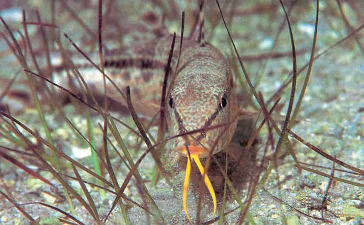
4
SEAGRASSES AND SEAWEEDS
4.1 INTRODUCTION
4.1.1 A brief history of research on seaweeds and
seagrasses of the region
The Red Sea has been a region of natural history exploration
by European scientists for more than 200 years. Previous to the
completion of the Suez Canal in 1869, travellers generally
started their journeys of exploration from one of two points.
From the east coast of Egypt (usually Suez), they could travel by
vessels to the Arabian coast and then on to the Ethiopian coast,
or they entered the Red Sea from the south, through the Strait of
Bab el Mandeb, coming by ship via the Cape of Good Hope.
After the completion of the Suez Canal many expeditions passed
through the Red Sea on their way to other parts of the Indian
Ocean. During that time numerous marine algae were collected,
resulting in the description of many species with the Red Sea as
type locality. A historical review of phycological research in the
Red Sea is given by PAPENFUSS (1968). The first record of
marine algae from the Red Sea dates back to 1756, and since
then there have been a number of important contributors to the
knowledge of the marine algae of the Red Sea. These include
Forsskål (18th century); Turner, Delile, Lamouroux, Decaisne,
Agardh, Montagne, De Notaris, Zanardini, Piccone, Hauck, and
Bornet (19th century); Reinbold, Lyle, Christensen, Børgesen,
101

---

Standard Survey Methods
Nasr, Newton, Rayss, and Dor (20th century).
in the world. Together the intertidal and
A milestone in macroalgal research in the Red
subtidal zones give rise to a narrow coastal
Sea was the catalogue and bibliography of the
area that accounts for less than one percent of
Red Sea benthic algae, compiled by
the Earth's surface. However the productivity
PAPENFUSS (1968). Recent studies include
of this region can equal or exceed that of most
WALKER (1987) and ATEWEBERMAN (1997).
terrestrial communities (DAWES 1998).
PRICE et al. (1988) studied the ecology of
seagrasses in the Red Sea. Global taxonomic
and biogeographical studies on seagrasses
Several areas with hard substrate in the
have been carried out by DEN HARTOG (1970)
Red Sea and the Gulf of Aden are not
and PHILLIPS & MEÑEZ (1988).
dominated by corals but by macroalgal
assemblages. Shallow coral reef areas of the
northern and central Red Sea are often
Very little is known about the seaweeds
dominated by filamentous greens, small
and seagrasses of the Gulf of Aden. ORMOND
browns and tuft-forming red algae. In
and BANAIMOON (1994) investigated the
upwelling regions (e.g. south coast of Yemen)
ecology of intertidal macroalgal assemblages
large brown algae may dominate. Perennial
on the Hadramaut coast of southern Yemen.
brown algae (such as Sargassum, Cystoseira
This study resulted in a list of 163 taxa of
and Hormophysa) are dominant over
seaweeds. WYNNE and JUPP (1998) compiled
extensive parts of shallow hard substrata in
74 new records of benthic marine algae for the
the southern Red Sea. In most of these areas
flora of Oman. More recently, the United
algal communities show a strong seasonality;
Nations Development Programme (UNDP)
many seaweed species appear to be annual.
has become involved in the conservation and
Seasonality is correlated with water
sustainable use of the biodiversity of the
temperature that, for the Red Sea, is coldest in
Socotra Archipelago (UNDP/GEF Project
winter but for the Arabian Sea, is coldest
YEM/96/G32). The seaweeds and seagrasses
during the summer upwelling (SHEPPARD et al.
of these islands have been studied by
1992; BANAIMOON 1998).
LELIAERT (1999), SCHILS (2000), WYNNE &
LELIAERT (2000), SCHILS (2002), SCHILS &
COPPEJANS (2002, 2003a, 2003b), SCHILS et al.
Seagrass communities
(2003a, 2003b). The seaweeds and seagrasses
Seagrass communities (also called
of the north coast of Somalia remain largely
seagrass beds or meadows) often characterise
unstudied.
sandy and muddy biotopes. Seagrasses are
monocotyledonous angiosperms adapted to
marine life both through their physiology and
4.1.2 An overview of the significance of
morphology. The most obvious characters of
seaweed and seagrass communities in the
seagrass species are the extensive rhizome and
region
rooting systems, and the very flexible,
generally strap-like leaves. Tropical seagrass
beds on mud, sand or coral rubble can consist
Seaweed communities
of a single species, but often contain members
Seaweeds can grow as individuals, but
of different genera. According to some
they more frequently live together in
phytosociologists, seagrass beds are the most
communities with other seaweed and animal
simply structured communities of rooted
species. Seaweed communities affect and are
plants, as they are mostly composed of only
affected by the environment and are some of
one or a few rooting species. This often gives
the most productive marine plant communities
seagrass meadows a rather monotonous
102

---

Seagrasses and Seaweeds
appearance. However, the structure of these
4.1.3 Species recorded in the area
apparently uniform seagrass beds disguises a
great diversity of floral and faunal
Seaweeds
components. Seagrass ecosystems provide
The catalogue of the Red Sea benthic
habitats for a wide variety of marine
algae by PAPENFUSS (1968) contains more
organisms, both plant and animal. These
than 500 seaweed taxa. The proportion of
include meiofauna and flora, benthic flora and
species endemic to the Red Sea is about nine
fauna, epiphytic organisms, plankton and fish,
percent. On the other hand, 64 percent of the
not to mention microbial and parasitic
species are pan tropical. WALKER (1987)
organisms. The relatively high rate of primary
separated the known species into four
production of seagrasses drives detritus-based
geographical regions, the gulfs (i.e. Gulf of
food chains, which help to support many of
Aqaba and Gulf of Suez), northern, central
these organisms. Birds, fishes and turtles also
and southern regions. He showed that the
directly consume seagrasses. Four main sub-
percentage of species known from the Red
habitats can be recognised in seagrass beds.
Sea that occur in any one of the four regions,
These are:
was between 8% and 40%. Many of the
southern species are typical of warm waters
The leaf epiphyton, comprising the
from the tropics, while the northern species
microflora with associated small
include members typical of slightly cooler
animals, including nematodes,
areas. The boundary between the two species
polychaetes and crustaceans, together
assemblages is drawn approximately through
with sessile fauna, such as hydroids
the middle of the Red Sea. The seaweeds of
and anemones, and larger animals,
the Gulf of Aden have been less well studied,
such as snails, echinoderms and small
especially from the north coast of Somalia.
fish;
From the south coast of Yemen, 163 seaweed
taxa have been recorded (O
Stem and rhizome biota, which include
RMOND
&
B
larger epiphytic algae, various
ANAIMOON 1994).
polychaetes, amphipods and bivalves;
Species swimming among the leaves
Seagrasses
including fish and crustaceans;
Ten species of seagrasses have been
recorded from the Red Sea. These belong to
Sediment fauna, although this may
seven genera, the total number known for the
differ little from that of the
tropical Indo-West Pacific region. On the
surrounding benthos.
eastern Red Sea coast, seagrass assemblages
have been identified from cluster analysis
The distribution and complexity of
using species cover data (PRICE et al. 1988).
seagrass habitats in the Red Sea and the Gulf
At a broad level, this revealed three groupings
of Aden is probably controlled by habitat
separated by latitude, suggesting
availability and extremes of temperature and
biogeographic trends. A more detailed study
salinity. Seagrass beds develop to their fullest
carried out in the southern Red Sea indicated
extent in the south of the Red Sea. This area is
six distinctive assemblages. Three of these
characterised by a wide and shallow shelf, a
were dominated by a single seagrass species
high prevalence of unconsolidated sediments,
(Thalassia hemprichii, Halophila ovalis and
and low temperature and salinity fluctuations
Halodule uninervis) (SHEPPARD et al. 1992).
(SHEPPARD et al. 1992). Limited areas of dense
seagrass beds have been recorded in the Gulf
of Aden (HIRTH et al. in SHEPPARD et al. l992).
103

---

Standard Survey Methods
4.2 METHODOLOGY
Braun-Blanquet's sociability scale
1 solitary
4.2.1 Qualitative assessment of the
macroalgal and seagrass flora of an area
2
in small groups or tufts
A qualitative assessment of the marine
3
in larger groups, cushions or humps
flora involves collecting specimens from a
4
in mats or very large groups
specific area, resulting in a list of species.
Depending on the study, the coastal area can
5
covering approx. the entire quadrat
vary from small (e.g. a coastal band of 10 m,
a rock outcrop, etc.) to large (e.g. one to
Table 4.2 The Braun-Blanquet's sociability scale
several kilometres of coastline, or a small
for the indication of a species' life form; after
S
offshore island). The resulting species list is
CHAMINÉE et al. (1995) and SCHILS (2000).
important for calculating biodiversity indices
for the area. When comparing species
Field collecting (intertidal and subtidal)
numbers or biodiversity indices for different
and preservation of marine plants
coastal areas, these areas should be of
Extensive and well-prepared collections
comparable size. A major disadvantage of
are the basis of all studies of marine
qualitative collection data is that species
organisms. The importance of good
abundance is not taken into account. This can
collections for taxonomic studies is evident,
be corrected, partially, by making the
but it is equally important that representative
sampling method semi-quantitative. This
collections ­ often referred to as `voucher
implies that each species is ranked based on
specimens' ­ be kept of each species recorded
its abundance, evaluated by visual
during an ecological survey. Without such
observations. An example of such a ranking is
specimens, there is little possibility of
the Tansley scale (Table 4.1). The growth
checking and confirming identification on the
form (sociability) of seaweeds can also be
basis of names used in publications. Such
taken into account. Here the Braun-Blanquet's
specimens should be numbered, labelled, and
sociability scale can be used for each species
deposited in a recognised herbarium
(Table 4.2).
(WOMERSLEY 1984).
Collecting. Intertidal habitats can be
Tansley scale
surveyed by wading during (extreme) low tide
d
dominant
or by snorkelling at high tide. Subtidal
c
co-dominant
collecting can be done by snorkelling or
a
abundant
scuba-diving. For the non-diver, subtidal
f
frequent
seagrass and algal beds can be sampled in
calm waters (at least down to several metres)
o
occasional
using a dredge. Whether making subtidal or
r
rare
intertidal collections, similar water-resistant
s
sporadic
equipment will be required. If wading,
Table 4.1 The Tansley scale, an indication of
collecting shoes, or boots should be available.
species abundance in a quadrat (quantitative
Many algae and some seagrasses can be
sampling) or larger area (semi-quantitative
removed by hand, but a scraper or a stout
sampling); after SCHAMINÉE et al. (1995) and SCHILS
knife may be necessary. A spade is useful in
(2000).
seagrass beds. Some thick encrusting algae
104

---

Seagrasses and Seaweeds
can be removed with a knife, but many
Herbarium sheets can be prepared directly
(especially the crustose coralline algae) must
in the field using fresh plant material or in the
be collected along with the substrate. This can
laboratory using material preserved in
only be done with heavy instruments such as
formalin. The preparation of fresh material
a hammer and chisel. Specimens can be kept
should be done as quickly as possible after
in a variety of field containers such as
leaving the field (preferably the same day)
buckets, (zip-) bags, perforated plastic bags or
because seaweeds die off very quickly. The
mesh bags. Small plastic vials can be useful
material is first sorted in plastic trays and
for minute specimens. The collected material
complete specimens (including the holdfast
should be kept in water to avoid decay by
and reproductive structures, if available) are
temperature rise or desiccation. Each
selected for preparation. These plants are then
container should be given a serial number on
mounted by "floating out". The specimen is
a water-resistant label, and recorded on a
immersed in a tray with seawater and
clipboard with waterproof paper or on a
arranged with forceps on an immersed sheet
scuba-board. Ecological data (intertidal zone,
of stiff herbarium paper on which the
substrate type (rock, epiphytic, sand, silt, etc.)
specimen number has been written in pencil.
and inclination (horizontal, vertical,
The herbarium sheet with specimen is
overhanging) should be noted for each
removed horizontally from the seawater,
collecting site. Additional information on
drained of the surplus water and deposited on
collecting seaweeds and seagrasses is given
newspaper, covered by a piece of cloth and a
by DAWES (1998), TSUDA & ABBOTT (in
newspaper again. A stack of herbarium sheets
LITTLER & LITTLER 1985), and WOMERSLEY
and newspapers is built up and placed in a
(1984).
plant press under moderate pressure. Adding
corrugated cardboard between stacks of
newspapers and specimens enhances drying.
Preservation.
Seagrass and algal
The newspapers must be changed at frequent
specimens can either be preserved in formalin
intervals (twice a day) until the specimens are
(wet preservation), or prepared on herbarium
dry.
sheets (dry preservation). Each specimen to
be preserved is given a serial number that
corresponds with a number in a notebook. The
Labelling. Unless specimens are properly
notebook contains the data recorded with each
and accurately labelled, they are of little
specimen; this information is placed on the
value. Data recorded with each specimen
label at a later stage (see below).
should include:
The locality (latitude and longitude are
Formalin is about 40% by volume
useful, especially for remote sites);
formaldehyde, and is diluted 1/10 with
seawater, giving a solution of 10% formalin or
Ecological notes, including the zone
4% formaldehyde (the concentration is not
(intertidal) or depth (subtidal), slope,
critical and half the above will usually give
exposed at low tide or submerged in an
good preservation). Formalin is a strong
intertidal pool, type of substrate,
irritant and carcinogenic so it should be
degree of wave exposure, temperature,
handled with care, avoiding inhalation or
etc.;
direct contact with the skin.
Notes on morphology such as colour
and texture;
105

---

Standard Survey Methods
Date;
observations. Surveys are particularly useful
for the study of large areas (e.g. kilometres of
Collector name(s);
coastline). The procedures are simple and
Collector number.
yield repeatable results in studies of seaweed
and seagrass communities. Ground-truth
Mounting dried specimens. The dried
observations can be carried out by qualitative
specimens are mounted on herbarium sheets
or quantitative assessment of the marine flora
of a standard format and the labels are added.
of the area. Quantitative assessment is carried
Specimens that do not stick on the paper
out using sample plots that are selected along
should be stuck with adhesive paper (not with
the coast based on visual observations. The
adhesive tape or glue).
combination of remote sensing and ground-
truth observations offers information for the
creation of vegetation maps. A concrete
Identification of seaweeds and seagrasses
example is given in DAHDOUH-GUEBAS et al.
No marine flora guides exist for the study
(1999).
area, hampering identification of seaweeds.
Some field guides from adjacent areas, which
may be helpful to identify the seaweeds of the
Remote sensing
Red Sea and the Gulf of Aden, are: JAASUND
Remote sensing uses sensors to identify or
(1976: Tanzania) and COPPEJANS et al. (1997:
measure parameters of an object according to
East Africa). Since 64% of the seaweed taxa
variations in the electromagnetic radiation
in the Red Sea are pan-tropical, floras or field
(EMR) reflected or emitted by the object.
guides from other tropical or subtropical
EMR can be natural, either reflected radiation
regions can be used, certainly for
from the sun or emitted heat from the earth. It
identification to genus level. These include
can also be man-made such as a radar system.
guides prepared by ABBOTT (1999: Hawaii,
The wavelength of electromagnetic radiation
red algae); COPPEJANS (1983: Mediterranean);
spans many orders of magnitude and is
CRIBB (1983: Australia, red algae); DE
conveniently divided into several arbitrary
CLERCK & COPPEJANS (1996: Jubail, Saudi
regions (e.g. ultra-violet, visible, near
Arabia); LAWSON & JOHN (1987: West Africa);
infrared, infrared, etc.). The amount and type
LITTLER & LITTLER (2000: Caribbean); SILVA
of radiation reflected or emitted depends upon
et al. (1996: Indian Ocean); TAYLOR (1960:
incident energy (e.g. thermal radiation) and
tropical eastern coast of America); TRONO
the nature of the earth's surface. Remote
(1997: Philippines).
sensing can be carried out by aerial
photography or scanning systems (airborne
spectral scanners or satellite sensors).
Seagrass identification can be carried out
GUILLAUMONT et al. (1997) discuss spectral
with DEN HARTOG (1970) or PHILLIPS &
properties of seaweeds in their natural habitat
MEÑEZ (1988).
and provide a critical review of sensors and
data processing for remote sensing of seaweed
communities. Methods for distribution and
4.2.2 Remote sensing combined with
mapping of seagrass communities using
ground-truth observations (phytosurvey)
remote sensing and ground-truth observations
are dealt with by KIRKMAN in PHILLIPS &
Survey techniques include creation of
MCROY (1990).
landscape and vegetation maps through
remote sensing (aerial photography or
scanning systems) and ground-truth
106

---

Seagrasses and Seaweeds
Aerial photography. Aerial photography
populations, are time consuming. Other
can be carried out from fixed-wing aircraft
methods include planimeter methods, grid
(light or medium altitude aircraft), or
count methods and scannerisation.
helicopters. Photography is carried out using
GUILLAUMONT et al. (1997) have reviewed
several types of photographic emulsions
data processing techniques. The most
simultaneously. Films are chosen according to
significant advances in the use of remote
their respective performances: colour and
sensing data are in the field of Geographical
infrared for intertidal, colour for submerged
Information Systems (GIS).
areas, colour and false colour film for floating
algae. Photographs have little spectral
capacities (infrared and visible field).
Ground-truth observations and creation
However, they provide high spatial resolution,
of vegetation maps
allowing texture analysis and good geometric
Once aerial photographs have been
quality.
examined, some form of ground-truth survey
must be carried out. Ground-truth
observations can be conducted through
Airborne spectral scanners. Image
qualitative or quantitative assessment (or a
spectrometers have a good to excellent
combination of the two) of the marine flora of
radiometric and spectral resolution but are
the area. Qualitative assessment implies
much more expensive than photographic
general collection over a large area: several
systems. They are also more expensive and
metres to kilometres of coastline. Quantitative
complex to use over large regions than
assessment implies selecting sample plots
satellite data.
(1­10 m2) along the coast (DAWES 1998).
The choice of location of the sample plots is
determined by the data from the remote
Satellite sensors. Satellite imagery
sensing. In these sample plots each dominant
provides reliable synoptic information
species is ranked for abundance, cover, and
reaching the user cheaply at regular intervals.
growth form (see 4.2.3. investigation of
It is a consistent and repeatable method.
spatial community variation ­ quadrat
Historical data are available since the 1970's.
sampling). The combination of data acquired
Radiometric calibration can be produced in
from remote sensing and ground-truth
good conditions. However, satellite sensors
observations can then be used to draw up
have limited performance in seaweed studies
vegetation maps.
because of their low spatial and spectral
resolution, frequency and sensitivity.
Moreover, bands are not optimal for
4.2.3 Quantitative sampling methods
underwater studies.
Investigation of spatial community
Data acquisition
variation
Qualitative images obtained from the
Transect sampling. Transects are used in
methods discussed above need to be
plant zonation studies of intertidal
transformed to quantitative information. This
communities (seaweeds) or where line
requires measurement of the areas covered by
quadrats are used (across seagrass beds).
the various identified populations. Different
Stakes are aligned from the highest to lowest
techniques have been developed. Classical
zone and a metric tape stretched between
methods, such as manual measurement of the
them. Samples for identification can be taken
areas covered by the various identified
along the transect in each zone, or at every
107

---

Standard Survey Methods
unit of measurement (every centimetre to
coastline). They can also be used in zonation
every few metres, depending on the slope and
studies to develop a more accurate
detail required). Percent species is determined
determination of percentage cover, frequency
by dividing the number of individuals within
and abundance.
a zone, by the total number present along the
entire transect. Percent species cover is
calculated by dividing the length (in
To avoid bias in sampling, random or
centimetres or metres) of the transect (or
haphazard methods can be used for quadrat
zone) species cover by the total length of the
placement. Figure 4.1 shows a fictional
transect (or zone).
example of a sample strategy to determine
changes in species composition along a
stretch of coastline. Quadrats can also be
Quadrat sampling. Measurements of
placed at regular intervals along each transect.
unit-area can be done using quadrats ranging
in size from 25 cm2 to 1 m2 squares; larger
or smaller areas can be used according to the
Species abundance in each quadrat can be
community structure and the accuracy
determined in a number of ways:
required. Determination of the quadrat size is
crucial. The frame size is a reflection of the
counting individuals of each species,
size of the patches in the population. For
instance, if seagrass shoots or seaweeds are
estimating cover of each species, or
clumped in 1 dm2
patches, frames
considerably larger (e.g. 1 m2) should be used
determining biomass (standing crop).
to ensure the inclusion of several patches.
Quadrat frames can be easily and
Other vegetation parameters that can be
inexpensively constructed from plastic pipe
recorded for the species in a quadrat are
(PVC works well). Quadrats may be
sociability and phenology. For sociability, the
subdivided if detailed sampling is required.
Braun-Blanquet's sociability scale can be
Quadrat samplers are useful to determine
used (Table 4.2). The phenology of a species
changes in species composition in areas with
can be indicated as: g = germling, v =
major shifts in abiotic factors (e.g. a
vegetative, f = fertile (if possible with
temperature gradient along a stretch of
indication of the life stage), dis = old thallus
parts remain, dth = thallus almost vanished.
infralitto ral
fring e
distance (km )
0
10
20
30
40
50
60
70
tem perature (°C )
24.0
24.2
24.5
24.8
25.2
25.5
25.8
26.0
Figure 4.1 Fictional example of a sample strategy to determine changes in species composition along a
stretch of coastline. Every 10 km, 5 quadrats (1 m2 each) haphazardly placed in the infra-littoral fringe are
examined. See text for explanation.
108

---

Seagrasses and Seaweeds
Counting the number of individuals of
each species can be problematic; in many
Braun-Blanquet's combined estimation
algal species individuals cannot be

No of individuals
Cover
distinguished as they grow in a diffuse
r very few <5%
manner forming algal tufts. Counting the
+ few
<5%
number of individuals in seaweed

communities should only be considered with
1 numerous
<5%
large distinct species, e.g. large browns.
2 very numerous >5%


Instead of absolute numbers, a scale, e.g. the
or arbitrarily
5 - 25%
Tansley scale (already mentioned in 4.2.1) can


3
arbitrarily
25 - 50%
be used (Table 4.1).

4
arbitrarily
50 - 75%
5
arbitrarily
75 - 100%
In seagrass communities, species
abundance is often determined by estimating
Table 4.3 Braun-Blanquet's combined estimation
the number of seagrass shoots in a quadrat.
of species abundance and cover; after SCHAMINÉE
et al. (1995) and SCHILS (2000).
Shoot density refers only to the above
ground, leafy portions of the plant. The
growth forms: e.g. crustose species, an algal
density of roots is correlated to the density of
turf layer overgrown by a layer of larger
shoots, but due to difficulty in measurement,
foliose or filamentous algae, overgrown by
is seldom quantified. Both destructive and
large fucoid algae or kelp. In such a case the
non-destructive means of estimating shoot
percentage cover of species is somewhat more
density can be used. A destructive technique
complicated to estimate. Moreover the total
commonly used involves clipping a quadrat of
cover (i.e. the sum of all species cover in a
shoots at the sediment surface and measuring
quadrat) can exceed 100%. Cover estimates
leaf surface area in the laboratory. The
can also be applied in seagrass beds but the
advantage of using destructive sampling is
estimation of shoot density is more widely
that samples can be processed in the
used (see above).
laboratory and leaf area (see leaf surface area
below) and biomass determination (see
below) can be conducted on the same sample.
Species abundance can also be determined
Non-destructive estimates of shoot density
by biomass or standing crop measurements.
allow for minimal perturbation of the
There are a number of ways of expressing
meadow, which is useful for repeated
biomass or standing crop: wet weight, dry
sampling (see investigation of temporal
weight, weight of organic carbon or inorganic
community variation below). Counting shoots
nitrogen.
within a quadrat can be accomplished at low
tide in intertidal meadows and with scuba
equipment in subtidal meadows (DENNISON in
The most widely used unit is dry weight in
PHILLIPS & MCROY 1990).
g/m2. Dry weight of seaweed and seagrass
species can be determined by oven-drying the
specimens at 70°C for 72 hours. To allow
Percentage cover can be estimated using
comparisons, this unit should be given
broad categories (e.g. a Braun-Blanquet's
whenever possible, specifying whether it
scale, Table 4.3). Seaweed communities are
applies to pure stands or to a larger area
often characterised by different layers of algal
including bare substrate patches. In the latter
109

---

Standard Survey Methods
case, the percentage-cover of the seaweed or
All data recorded in each quadrat should
seagrass bed in the area considered should be
be written down in a standardised format.
noted. If only wet weight can be determined
Table 4.4 shows an example of such a data
routinely, at least one series of wet weight/dry
entry form.
weight (wwt/dwt) correlations per dominant
species should be made, since this ratio may
vary considerably between different seaweed
Specific techniques for the investigation of
and seagrass species according to the texture
seagrass communities
of the plant tissue.
Root/shoot ratios (R/S) (FONSECA,
THAYER & KENWORTHY in PHILLIPS & MCROY
1990). The R/S ratio has been used
Date Hour
Tidal
coefficient
Place
GPS position

Quadrat No.
Depth
Intertidal zone
Photo

No Species
Br.-Bl.
Phen. Soc. Tans.
w.w.
(g)
1.





2.





3.





4.





5.





6.





7.





8.





9.





10.





etc






Animals:


Additional observations:


Sal.
Temp.
Nutrient container no.
Secchi Slope
Sand
cover
Table 4.4 Example of a macroalgal vegetation sampling sheet. Species cover is estimated and wet weight is
determined in the field. Some environmental variables are measured on site and a sample of seawater is collected
for nutrient analysis. Br.-Bl.: Braun-Blanquet's combined estimation (Table 4.3); Phen.: phenology; Soc.:
sociability (Table 4.2); Tans.: Tansley scale (Table 4.1); w.w.: wet weight in grams; Sal.: salinity measured with
a refractometer; Temp.: temperature measured with a glass thermometer; Secchi: water transparency (in cm)
measured with a Secchi disc; Slope: estimation of the slope in degrees; Sand cover: estimation of the percentage
sand cover in the quadrat; after SCHILS (2000).
110

---

Seagrasses and Seaweeds
operationally to include both root and rhizome
Static measures (one point in time) of
components. R/S ratios are relatively simple
seagrass R/S ratios can be used to assess the
to measure and enhance estimates of total
degree of development of a seagrass system.
production by seagrass species. R/S ratios
Because some seagrass components take a
should be derived from plant material
long time to decompose, it is necessary to
separated into shoot and root (plus rhizome)
quantify living versus dead material. An older
components at the meristem where cell
seagrass meadow generally has a lower ratio
differentiation occurs. R/S ratios are usually
of living to dead seagrass components
presented on a weight/weight basis, although
(especially roots and rhizomes). For foliar
area and volume ratios can also be
portions, a visual examination of the shoot
determined. Weight data should be presented
will suffice to distinguish living green blades
on an ash-free dry-weight basis, since
from dead ones. For roots and rhizomes, a
inorganic contamination may account for up
visual plus a physical examination is needed.
to 50% of the dry weight. The leaves and roots
Most roots decompose relatively quickly
should be placed in 5% phosphoric acid for
compared with rhizomes and will no longer
10­15 minutes to remove carbonates and
appear white or succulent after senescence.
encrusting epiphytic organisms, and then
Rhizomes may appear to be intact, but flexing
rinsed in tap water. Plant components should
the rhizome to the point of breaking should
then be dried in an oven at 80°C. Subsamples
produce a brisk snap if it is still alive.
of the dried plant material should be ashed at
550°C for 4­6 hours to determine ash-free dry
weight (AFDW). Field methods for R/S
Leaf surface area (BULTHUIS in PHILLIPS
collections may vary depending on the
& MCROY 1990). The leaf area of seagrasses
required precision and accuracy. Clipping
in a quadrat must be known in order to
shoots out of a quadrat at the sediment surface
calculate the leaf-area index (one-sided leaf
will suffice for above-ground estimates.
area per unit ground area), and to calculate
Running a sharp blade around the inside edge
photosynthesis (moles of carbon or oxygen
of the quadrat and harvesting the portions of
per unit leaf area). Leaf area can be measured
the plant in the sediment provides the below-
directly using an area meter, planimeter or
ground part for the ratio. This method may
digitiser, calculated from length, width and
well leave some deeply rooted material
diameter measurements. The easiest and most
behind (e.g. Thalassia roots can extend 4 m
accurate method of measuring leaf area,
into the sediment). Usually, however, the
irrespective of whether leaves are linear or
majority of root and rhizome is found in the
irregularly shaped, is by using an area meter
upper 20­40 cm of the sediment.
(e.g. LICOR LI­3100). This instrument is an
automatically integrating planimeter
developed for measuring leaves. If an area
Wide variations in the R/S ratio occur
meter is not available the alternative method
among habitats as well as throughout the year.
chosen depends on leaf shape and the number
These are related to seagrass development
of leaves to be measured. Most seagrasses
processes and to prevailing environmental
have flattened, linear leaves so that leaf area
conditions. Seasonal changes in weight also
can be estimated by measuring length and
occur. Hence, there is an age-dependent
width. The width is measured at three or more
mechanism contributing to the rate,
locations along the leaf. The area is calculated
proportions and mass of observed R/S ratios,
by multiplying length by mean width.
causing these values to change with time.
111

---

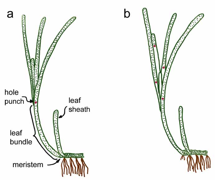
Standard Survey Methods
Leaf production (DENNISON in PHILLIPS &
marks made above the region of cell
MCROY 1990). The principal methods of
elongation can be used as a measure of leaf
measuring leaf production are by change in
growth. Several techniques of leaf marking
standing stock over time and by leaf-marking
have been employed. One method involves
techniques. The first method is problematic
stapling individual leaves. This marking
with seagrasses because of their perennial
technique is fast and easy but requires
growth and the loss of leaf material during
relatively large leaves. Several modifications
growth due to rapid leaf turnover.
of the staple technique have been developed
for seagrasses with small leaves. A small wire
inserted into the leaf, hole punches, or a
Leaf-marking techniques can be used to
water-insoluble pen can be used to mark
distinguish leaf tissue formed before and after
seagrass leaves (Figure 4.2). Marking with a
marking due to the growth form of seagrasses.
pen has the advantage of minimal damage to
Seagrass leaves have a basal meristem, which
the leaf. The time interval between marking
is near the sediment surface for most species.
and collection is constrained by the growth
Above this region of dividing cells is a region
rate of the plant, and the leaf turnover time
of elongating cells, which are usually
sets the upper limit.
protected by leaf sheaths. Above the dividing
and elongating cells, leaf tissue moves away
from the basal meristem as long as leaf
Several leaf production values can be
growth occurs, even though no cell division or
calculated from leaf-marking techniques. Leaf
elongation occurs in this region. Hence, the
material can be separated into leaf tissue
distance between the basal meristem and leaf
produced before (above mark) and after
Figure 4.2 Hole-punch method of leaf marking in which a syringe needle hole is created several centimetres
above leaf bundle (a) and the resultant scars used to distinguished leaf tissue which arose from the leaf before
(stippled) and after (unstippled) marking (b); after DENNISON in PHILLIPS & MCROY (1990).
112

---

Seagrasses and Seaweeds
marking (below mark and unmarked leaves),
primary production. The oldest of these
dried for 24 hours at 80°C and weighed. The
methods involves monitoring increase in plant
ratio of leaf material produced after marking
biomass over a growing season. Direct
to that present before marking, divided by the
measurements of changes in dissolved oxygen
time interval, yields a relative production rate
(O2) and dissolved inorganic carbon (DIC) in
(e.g. g g­1 day­1). For each shoot the leaf
water surrounding seaweeds or seagrasses
material produced after marking divided by
have been used successfully for various
the time interval yields leaf production per
macrophyte systems. The radioactive C14
shoot (e.g. mg shoot­1 day­1).
technique has had widespread use for
measuring seaweed and seagrass production.
For a description of the different techniques to
Investigation of temporal community
measure primary production we refer the
variation
reader to KEMP, MURRAY & MCROY in
In order to investigate the temporal
PHILLIPS & MCROY (1990); ARNOLD &
variation of seaweed and seagrass
LITTLER in LITTLER & LITTER (1985); and
communities, permanent quadrats (PQ) can be
KENNISH (1989).
used. The methods used in this survey
technique are explained by POLDERMAN in
PRICE et al. (1980). In principle, the
4.2.4 Measurement of environmental
procedures for a general survey (e.g. quadrat
variables
sampling as explained above) and for the
monitoring of one particular station
(permanent quadrat sampling) are the same,
Water temperature
the difference being that the latter procedure
It has been shown that individual seaweed
is repeated at regular time intervals. The
species distributions over a biogeographic
choice of time interval depends on the
scale are overwhelmingly limited by seawater
objective of the investigation. If, for example,
temperature regimes. In the ideal situation,
the study is to determine seasonal changes in
temperature should be recorded continuously
species composition, then the permanent
or several times a day in order to calculate
quadrats should be examined at least once a
minimum, maximum and average
month. Quadrats measuring from 25 cm2 to
temperatures per day, month and year. If daily
1 m2 are placed in a homogeneous vegetation
temperature recording is not possible, it
patch. The different measurements for species
should be recorded at regular time intervals
abundance used in the quadrat sampling can
(e.g. once a month) over several years.
also be used here.
Temperature varies with water depth, currents
and waves, the amount that seaweeds or
seagrasses retard water motion, as well as
Primary productivity
with local insolation. It is recommended that
In any study of seaweed or seagrass
the temperature be measured near the
ecology or physiology, a measurement of
substrate at different water depths.
fundamental interest is the primary production
Temperature should be recorded using the
of the population or community. Carbon fixed
Celsius scale. A glass thermometer, protected
in photosynthesis, and organic matter
in a steel case, can be used for these
accumulated with plant growth, constitute the
measurements. For many studies,
very basis for the seaweed or seagrass
combination sensors recording temperature as
community, its physical structure, its food
well as salinity or conductivity simplify in situ
supply and its mineral cycle. Numerous
measurements.
techniques are available for measuring
113

---

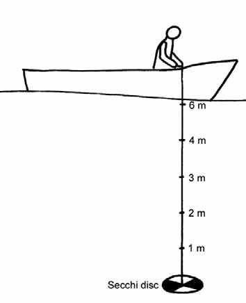
Standard Survey Methods
conversion factors may be derived by taking a
number of simultaneous readings above and
below the water. Total irradiance under water
is measured by immersing a radiometer or
quantum meter at the appropriate depth.
Shore height
Shore height above the low water mark
(mean or extreme low tide) is measured using
a level meter (or theodolite) and a surveyor's
rod (Figure 4.4). Height is measured relative
to the low water mark on a specific day and
time. These relative measurements have to be
transformed to absolute measurements by
using tide tables and curves. For example in
Figure 4.4 the height of plot 1 relative to the
extreme low water mark is b ­ a1 + c.
Figure 4.3 Use of a Secchi disc to measure water
transparency. The Secchi disc is lowered in the water
until it disappears from the view of a human
observer. This depth is a measure for water
Depth
transparency, which is in its turn a measure for light
Depth below low water mark can be
penetration to the bottom.
measured using a depth sounder on board a
vessel, or a depth meter while scuba-diving.
Light
The measurement of the sun's energy for
photosynthesis is complex under any
Sand inundation
circumstances. The complexity is
Sand inundation can be determined by
compounded when the light is filtered through
estimating the percentage of sand cover in a
water. Different measurement techniques
quadrat or by removing all sand in a quadrat
(such as Secchi disc measurements, hours of
and measuring the wet or dry weight.
daylight, total solar radiation and total
irradiance under water) can be used in
combination. The simple long-standing
Substrate
Secchi disc method measures the depth at
Seaweeds grow on different types of
which light, reflected by the Secchi disc,
substrate including rock, fossil coral, or
disappears from the view of a human observer
artificial substrates such as plastic buoys or
as the disc is lowered into the water (Figure
wooden constructions. Type as well as texture
4.3). Measurement of the hours of daylight are
of the substrate should be determined.
useful when making comparisons over many
Seagrasses grow on sand or mud flats. Here
years of overall light conditions that may have
the substrate type is determined by measuring
contributed to the presence, growth, or
particle size. This is done by taking a core of
disappearance of a seaweed or seagrass bed.
the sediment, which is dried, and then sieved
Total solar radiation is measured on land,
using a set of standard screens (0.063 mm to
usually with a pyrhelliometer. Daily
2 mm pore size). Particle-size distribution is
measurements may be available from a nearby
obtained by dividing the dry weights of each
installation, such as a marine station. To relate
size class by the total dry weight of the sample.
these data to underwater measurements,
114

---

Seagrasses and Seaweeds
1
2
3
a
a
a
b
plot 3
plot 2
LW
plot 1
c
ELW
Figure 4.4 Use of a level meter and surveyor's rod to measure shore height above low water mark (LW);
see text for explanation (ELW = extreme low water mark).
Slope
associated with storm events are among the
This should be measured in degrees: 0°
primary sources of variation to consider in
(horizontal) ­ 90° (vertical) ­ 180°
designing a sampling protocol for a given site.
(overhanging substrate). Instead of numerical
values, broad categories can be used (e.g.
horizontal, sub-vertical, vertical, overhang).
Nutrients
Four primary elements necessary for plant
growth are oxygen, carbon, nitrogen and
Water movements
phosphorus. Nitrogen and phosphorus can be
Waves, tides and currents can be
limiting nutrients to marine plants. Sample
important factors determining the structure of
and analytic methods for determining nutrient
a seaweed or seagrass community. Different
concentration are elaborate and will not be
types of measurement include cumulative
discussed here. The reader is referred to
water motion, maximum force and continuous
WHEELER in LITTLER & LITTLER (1985) for a
measurement of water velocity. An overview
review of analytical techniques.
of techniques is presented by Denny in
LITTLER & LITTLER (1985).
4.3 DATA ANALYSIS
Salinity
Salinity can be measured using a
Different sample methods require
refractometer. Refractometers are small and
different analysis techniques. This section
portable and give reliable readings.
focuses on the analysis of data collected to
Measurements of salinity do not generally
assess structural patterns in seaweed and
suffer from the daily variations experienced
seagrass vegetation, and spatial or temporal
by water temperature except for smaller
community variation.
intertidal pools (evaporation versus rain).
Rather, seasonal variation and changes
115

---

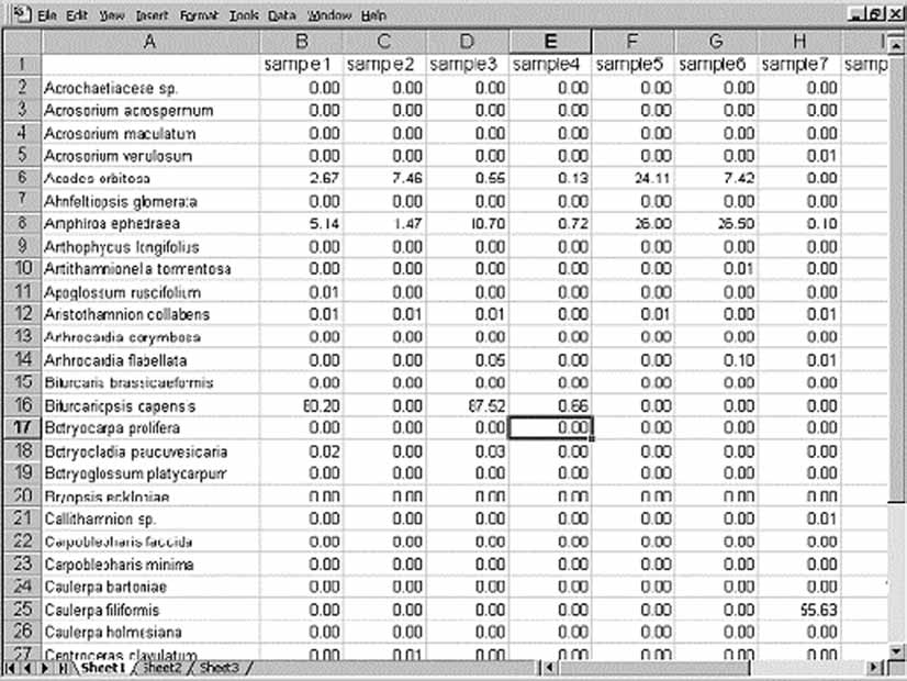
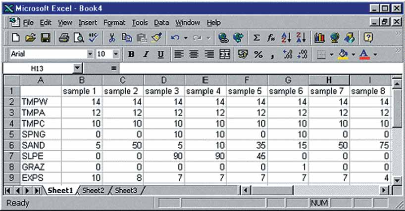
Standard Survey Methods
a)
b)
Table 4.5 Example of a matrix with species data (a), and environmental data (b), in an EXCEL spreadsheet.
See text for explanation. In the second matrix abbreviations are used for the environmental variables: temperature
variables (average temperature of warmest month, average year temperature, average temperature of coldest
month) (°C), sponge cover (%), sand cover (%), slope (°), grazers (number of grazing animals), exposure rate.
116

---

Seagrasses and Seaweeds
4.3.1 Sample data input: spreadsheets
patterns in data (e.g. structural and
and databases
distribution patterns) are ordination and
classification. An overview of multivariate
In order to analyse collected data, it must
analysis techniques in vegetation studies is
be entered in a data matrix. This can be done
given by KENT & COKER (1992).
in a spreadsheet or a database programme. In
the case of quadrat sampling, sample plots are
placed in columns and species in rows. The
Transformation of data
species abundance values can be
The number of species is usually not
presence/absence values, cover estimates,
evenly distributed over the plots. This is
biomass data, etc. If environmental variables
problematic for the implementation of
are incorporated in the analysis, they should
statistical techniques. Transformation of data
be placed in a second matrix: sample plots in
is a technique to correct this. Likewise,
columns, environmental variables in rows.
environmental variables can be transformed.
Table 4.5 shows an example of a species and
The question of optimal transformation of
environmental data matrix.
species abundances in ordination has not yet
been fully addressed. Techniques such as
Detrended Correspondence Analysis (DCA)
4.3.2 Preliminary data analysis:
and Canonical Correspondence Analysis
exploratory data analysis by means of
(CCA) appear to work well for raw data
descriptive statistics
values (e.g. percentage cover, biomass,
presence/absence data etc.) as well as for data
Descriptive statistics can be defined as the
values following logarithmic transformations,
enumeration, organisation and graphic
square root transformation, or transformation
presentation of data (data reduction).
into a traditional cover-abundance scale.
Preliminary data exploration can be done with
Apart from the problem of normal distribution
a simple spreadsheet programme or with
of data, logarithmic and square root
statistical programmes (e.g. STATISTICA®).
transformation are often used to dampen the
Simple graphs can often clarify the large and
effects of dominant species.
disorderly amount of data. Questions that can
be answered with descriptive statistics
include: what are the dominant species; what
Ordination
is the distribution of the dominant species;
Ordination is a widely used family of
what is the minimum, maximum, average and
methods, which attempt to reveal the
standard deviation of the environmental
relationships between ecological
variables; which locations are species rich or
communities. These multivariate techniques
species poor, etc.
arrange sites along axes on the basis of
species composition. The mathematical
theory behind the different ordination
4.3.3 Multivariate statistics
techniques is quite complicated. A
comprehensive overview of ordination
Studies in environmental biology usually
techniques used in community analysis can be
involve more than one variable (e.g. large
found in KENT & COKER (1992).
number of species, plots and environmental
variables). Analytic techniques that deal with
such kind of data are called multivariate
Indirect ordination methods arrange sites
analysis techniques or multivariate statistics.
along axes only on the basis of species
Techniques that are effective in revealing
composition. Widely used methods in
117

---

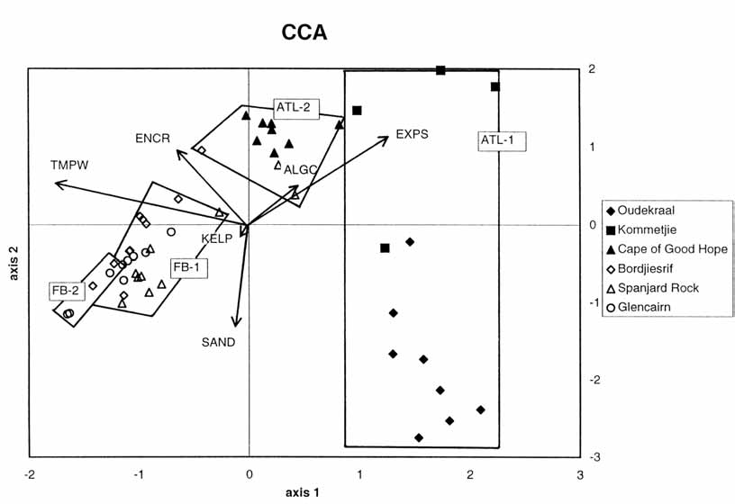
Standard Survey Methods
community studies are Principal Component
grouped together are characterised by similar
Analysis (PCA), Correspondence Analysis
species composition and environmental
(CA) and DCA. In direct ordination methods
conditions. Samples that are plotted far away
the arrangement of the sites is constrained by
from each other have very different species
environmental factors, which are incorporated
composition. Correlations can be examined
in the analysis along with the species
between environmental variables, species and
composition. Widely used methods are CCA
plots.
and Redundancy Analysis (RDA). The choice
of environmental variables greatly influences
the outcome of CCA and other constrained
Numerical classification
ordinations. For an exploratory analysis, one
Agglomerative methods (cluster analysis)
should certainly include variables that are
proceed from individual samples or quadrats
related to the most important determinants of
and progressively combine them in terms of
species composition. However, it is also often
their similarity in species composition until all
desirable to include other variables that are
the quadrats are in one group. The
easy and inexpensive to measure ­ one may
combinations are made by similarity
be surprised and find out that previously
coefficients that measure how alike any two
unsuspected factors are quite important in
quadrats are in terms of species composition
determining species composition
or by dissimilarity coefficients that assess
(PALMER 1993).
how unalike any two quadrats are. Different
cluster methods are used in community
studies: single-, complete-, and average-
The final result of an ordination is a two-
linkage clustering. A much-used similarity
dimensional diagram with samples, species
index in plant community studies is the
and environmental variables plotted
squared Euclidean distance. An overview is
(Figure 4.5). In simple terms, samples that are
given by KENT & COKER (1992).
Figure 4.5 An example of an ordination diagram in a study of subtidal algal community variation; after
LEILERT et al. (2000).
118

---

Seagrasses and Seaweeds
T r e m a t o c a r p u s f l a b e l l a t u s
C o d i u m s t e p h e n s i a e
B o t r y o c a r p a p r o l i f e r a
C h a m p i a c o m p r e s s a
B o t r y o g l o s s u m p l a t y c a r p u m
A m p h i r o a e p h e d r a e a
A t l
F B
C o d i u m s t e p h e n s i a e
C a u l e r p a f i l i f o r m i s
B o t r y o c a r p a p r o l i f e r a
P l o c a m i u m c o r a l l o r h i z a
P l o c a m i u m c o r a l l o r h i z a
B i f u r c a r i o p s i s c a p e n s i s
R h o d y m e n i a n a t a l e n s i s
T a y l o r i e l l a t e n e b r o s a
T r e m a t o c a r p u s f l a b e l l a t u s
C e r a m i u m p l a n u m
P o l y o p e s c o n s t r i c t u s
A t l - 1
A t l - 2
F B - 1
F B - 2
P l o c a m i u m s u h r i i
A m p h i r o a e p h e d r a e a
N e u r o g l o s s u m b i n d e r i a n u m
A r t h r o c a r d i a f l a b e l l a t a
E p y m e n i a c a p e n s i s
G i g a r t i n a
E p y m e n i a
A c r o s o r i u m
T r e m a t o c a r p u s f r a g i l i s
B o t r y o g l o s s u m p l a t y c a r p u m
b r a c t e a t a
c a p e n s i s
A e o d e s o r b i t o s a
v e n u l o s u m
A t l - 1 . 1
A t l - 1 . 2
A t l - 2 . 1
A t l - 2 . 2
1
A t l - 2 .
F B - 1 . 1
F B - 1 . 2
A c r o s o r i u m
R h o d o p h y l l i s
C a u l e r p a b a r t o n i a e
C l a d o p h o r a
P o l y o p e s
P t e r o s i p h o n i a
a c r o s p e r m u m
r e p t a n s
C . h o l m e s i a n a
m i r a b i l i s
c o n s t r i c t u s
c l o i o p h y l l a
F B - 1 . 1 . 1
F B - 1 . 1 . 2 A e o d e s
P l o c a m i u m r i g i d u m
R h o d o p h y l l i s r e p t a n s
o r b i t o s a
s
s a m p l e
1 .
1 1
1 .
1 8
2 .
2 2
2 .
2 3
2 .
2 4 1 .
1 2 1 .
1 5
1 .
1 7
2 .
2 1
1 .
1 6
1 .
1 3
1 .
1 4
3 .
3 6
3 .
3 7
3 .
3 8
3 .
3 1 3 .
3 2
3 .
3 3
3 .
3 4
3 .
3 5
4 .
4 6
5 .
5 6
5 .
5 7
5 .
5 3
5 .
5 4
5 .
5 5
4 .
4 3
6 .
6 1
6 .
6 2
6 .
6 3
6 .
6 4
6 .
6 5
6 .
6 6
5 .
5 1 5 .
5 2 5 .
5 9
5 .
5 1 0
5 .
5 8
4 .
4 2
4 .
4 4
4 .
4 5
4 .
4 7
6 .
6 8
4 .
4 1 4 .
4 8
4 .
4 9
4 .
4 1 0
6 .
6 7
6 .
6 9
Figure 4.6 An example of a TWINSPAN classification using the same plots as in the ordination of Figure 4.5;
after LEILERT et al. (2000).
Divisive methods start with the total
4.3.4 Calculation of species richness
population of individuals and progressively
divide them into smaller and smaller groups.
Biodiversity indices are an overall
Two-way indicator species analysis
measure of diversity that usually combine
(TWINSPAN) is now the most widely used
aspects of species richness and evenness.
technique for divisive classification in plant
Species richness is the number of species in a
community studies. The method is based on
given area. Evenness, or equitability, is the
progressive refinement of a single axis
uniformity of abundance in an assemblage of
ordination from reciprocal averaging or
species. Equitability is greatest when species
correspondence analysis. The output of a
are equally abundant. Two commonly used
TWINSPAN is a computer generated two-
indices used to express biodiversity are the
way table, which can be transformed into a
Simpson index and the Shannon-Weaver
classification (Figure 4.6). For each group of
(Weiner) index.
sample plots indicator species (i.e. species
typical for a group of plots) are defined.
Simpson's index assumes that the
proportion of individuals in an area
An overview of classification techniques
adequately weighs their importance to
used in community analysis can be found in
diversity. The equation for this index is:
KENT & COKER (1992).
D = 1­(sum (pi2))
When groups of plots can be clearly
distinguished (from ordination and
classification analysis), they indicate distinct
where D is the diversity and pi is the
community types, each being characterised by
proportion of the `i'th species in the total
its typical species composition and
sample. Values for D can range from one to
environmental variables.
the total number of species (S). An index of
one indicates that all of the individuals in the
119

---

Standard Survey Methods
area belong to a single species. When D = S
a high species turnover between adjacent sites.
then every individual belongs to a different
Gamma diversity or regional diversity is the
species and species are equally abundant.
diversity of a landscape, or all sites combined.
The Shannon-Weaver index is very similar
Different types of curves are utilised in
to the Simpson index, except for the
the visualisation of species diversity. A
underlying distribution. The Simpson index
species-individual curve is a plot of the
assumes that the probability of observing an
cumulative number of species encountered,
individual is proportional to its frequency in
versus the cumulative number of individuals
the habitat whereas the Shannon-Weaver
captured. A species-area curve is a plot of the
index assumes that the habitat contains an
(cumulative) number of species encountered,
infinite number of individuals. The equation
as a function of area. Species-area curves can
for this index is:
be used to compare different regions.
H = ­sum(pi ln(pi))
4.3.5 Computer software
This section gives a short overview of
H is high when equitability and species
existing software available for the above-
number are high.
mentioned analytic techniques.
The terms alpha, beta and gamma
Construction of data matrices
diversity are used to refer to biodiversity on
These can either be done in a spreadsheet
different spatial levels. Alpha diversity, or
or database programme. MICROSOFT EXCEL
local diversity, is the diversity within a site or
can be used as a spreadsheet programme,
quadrat. Beta diversity is determined to
MICROSOFT ACCESS as a database. MICROSOFT
measure the rate of species turnover between
EXCEL can also be used for exploratory data
adjacent sites or areas. Beta diversity can be
analysis (i.e. descriptive statistics and graphic
defined as a measure of how different (or
presentation) and transformation of data.
similar) a range of samples are in terms of
variety of species found in them (MAGURRAN
1988). A widely used method for measuring
Descriptive statistics and graphic
beta diversity using presence and absence data
presentation
is the Wilson and Shmida measure, T:
These can be carried out with a large
variety of statistical software packages. Two
widely used programmes are STATISTICA and
T = [g(H) + l(H)] / 2
SPSS.
Ordinations
where g(H) is the number of new species
Ordinations can be carried out with the
encountered and l(H) the number of species
FORTRAN programme CANOCO (TER BRAAK
which are lost along a transect; is the
1988). This programme offers many
average sample richness (i.e. average species
possibilities but it is not easy to use. More
number per area). A high T number indicates
recently, Windows versions of this program,
120

---

Seagrasses and Seaweeds
which are much more user-friendly, have
Cluster analysis
become available. A complete overview of
This can be carried out with statistical
ordination software can be found at
programs such as STATISTICA and SPSS. When
www.okstate.edu/artsci/botany/ordinate
using STATISTICA, cluster diagrams are directly
/software.htm. Two software packages will be
displayed. A demonstration version of
discussed below.
STATISTICA
can be downloaded from
www.statsoftinc.com/. A
demonstration
version of SPSS can be downloaded, from
CANOCO FOR WINDOWS 4.5, developed by
www.spss.com/.
the Centre for Biometry, Wageningen, offers
the same possibilities as the FORTRAN
programme but is much easier to use. A
Divisive classification
disadvantage of CANOCO is that it cannot
Divisive classification can be carried out
directly display ordination diagrams.
with the FORTRAN programme TWINSPAN (HILL
Therefore another program: CANODRAW 3.1 is
1979). No Windows version of this
used. The software can be ordered from
programme is yet available.
www.microcomputerpower.com/cfw/.
TWINSPAN, written by Mark Hill, is a
PC­ORD, a programme developed by
programme for classifying species and
Bruce McCune, offers a wide variety of
samples, producing an ordered two-way table
multivariate statistical analysis methods for
of their occurrence. The two-way table
ecological communities, including cluster
generated by the programme has to be
analysis, ordination, and species diversity.
transformed to a classification by hand. The
PC­ORD is an easy-to-use programme that
software package can be ordered from
directly displays ordination diagrams.
www.ceh.ac.uk/.
121

---

Standard Survey Methods
4.4 REFERENCES
Sanctuary, Saudi Arabia. In: A Marine
Wildlife Sanctuary for the Arabian Gulf.
Environmental Research and Conservation
ABBOTT, I.A. 1999. Marine Red Algae of the
Following the 1991 Gulf War Oil Spill.
Hawaiian Islands. Bishop Museum Press,
(Krupp, F., Abuzinada, A. & Nader, I. eds):
Honolulu. 477 pp.
199­289. Forschungsinstitut Senckenberg,
Frankfurt a.M. 675 pp.
ATEWEBERMAN, M. 1997. Taxonomic and
ecological study of benthic marine
DEN HARTOG, C. 1970. The sea-grasses of the
macroalgae of the Red Sea coast of Eritrea.
world. Verhandelingen der Koninklijke
Unpublished MSc. Thesis. 42 pp.
Nederlandse Akademie van Wetenschappen,
Afdeling Natuurkunde 2de reeks 59: 1­275.
BANAIMOON, S.A. 1998. Some biological
events associated with upwelling in the
GUILLAUMONT, B., BAJJOUK T. & TALEC, P.
Arabian Sea. In: Soqotra. Proceedings of the
1997. Seaweeds and remote sensing: a critical
First International Symposium of Soqotra
review of sensors and data processing. In:
Island: Present & Future. (Dumont, H.J. ed).
Progress in Phycological Research
Vol. 1: 233­246. United Nations Publications,
12: 213­282. (Round, F.E. & Chapman, D.J.
New York.
eds). Biopress Ltd., Bristol.
COPPEJANS, E. 1983. Iconographie d'algues
HILL, M.O. 1979. TWINSPAN ­ a FORTRAN
Méditerranées. Chlorophyta, Phaeophyta,
program for arranging multivariate data in
Rhodophyta.
Bibliotheca Phycologica
an ordered two-way table by classification of.
63:1­28.
the individuals and attributes. Cornell
University, Ithaca, New York. 52 pp.
COPPEJANS, E., RICHMOND, M.D., DE CLERCK,
O. & RABESANDRATANA, R. 1997. Marine
JAASUND, E. 1976. Seaweeds in Tanzania: A
macroalgae. In: A Guide to the Seashores of.
Field Guide. University of Tromsø, Tromsø.
Eastern Africa and the Western Indian Ocean
160 pp.
Islands. (Richmond, M.D. ed.): 70­95.
Swedish International Development Co-
KENNISH, M.J. 1989. Practical Handbook of.
operation Agency (SIDA), Department for
Marine Science. CRC Press, Boca Raton.
Research Co-operation, SAREC.
710 pp.
CRIBB, A.B. 1983. Marine Algae of the
KENT, M. & COKER, P. 1992. Vegetation
Southern Great Barrier Reef. Part I.
Description and Analysis: a practical
Rhodophyta. Brisbane, Australian Coral Reef
approach. CRC Press, Boca Raton.
Society. 173 pp.
LAWSON, G.W. & JOHN, D.W. 1987. The
DAHDOUH-GUEBAS, F., COPPEJANS, E. & VAN
Marine Algae and Coastal Environment of.
SPEYBROEK, D. 1999. Remote sensing and
Tropical West Africa (2nd ed). J. Cramer,
zonation of seagrasses and algae along the
Berlin. 415 pp.
Kenyan coast. Hydrobiologia 400: 63­73.
LELIAERT, F. 1999. Marine benthic macroalgae
DAWES, C.J. 1998. Marine Botany. 2nd Ed.
and seagrasses of the Socotra Archipelago. In:
John Wiley & Sons, Inc. New York. 48 pp.
Conservation and Sustainable Use of.
Biodiversity of Socotra Archipelago. Marine
DE CLERCK, O. & COPPEJANS, E. 1996.
Habitat, Biodiversity and Fisheries Surveys
Marine algae of the Jubail Marine Wildlife
and management. Report of Phase II. (Hariri,
122

---

Seagrasses and Seaweeds
K.I. & Krupp F. eds). Senckenberg Research
PRICE, J.H., IRVINE, D.E.G. & FARNHAM, W.F.
Institute, Germany. 12 pp.
1980a. The Shore Environment, Vol. 1:
Methods. Academic Press, London. 321 pp.
LITTLER, D.S. & LITTLER, M.M. 2000.
Caribbean Reef Plants. An Identification
PRICE, J.H., IRVINE, D.E.G. & FARNHAM, W.F.
Guide to the Reef Plants of the Caribbean,
1980b. The Shore Environment, Vol. 2:
Bahamas, Florida and Gulf of Mexico.
Ecosystems. Academic Press, London. 945 pp.
Offshore Graphics Inc., Washington. 542 pp.
SCHILS, T. 2000. Short Report: Macroalgal
LITTLER, M.M. & LITTLER, D.S. 1985.
assemblages of the Socotra Archipelago,
Handbook of Phycological Methods.
Yemen. In: Conservation and Sustainable Use
Ecological Field Methods: Macroalgae.
of Biodiversity of Socotra Archipelago. Marine
Cambridge University Press, Cambridge.
Habitat, Biodiversity and Fisheries Surveys
617 pp.
and management. Report of Phase IV. (Hariri,
K.I. & Krupp, F. eds). Senckenberg Research
MAGURRAN, A. 1988. Ecological Diversity
Institute, Germany. 12 pp.
and its Measurement. Princeton University
Press. 192 pp.
SCHILS, T. 2002. Macroalgal assemblages of the
Socotra Archipelago. In: Conservation and
ORMOND, R.F.G. & BANAIMOON, S.A. 1994.
Sustainable Use of Biodiversity of Socotra
Ecology of intertidal macroalgal assemblages
Archipelago. Marine Habitat, Biodiversity and.
on the Hadramout coast of southern Yemen,
Fisheries Surveys and Management. Final
an area of seasonal upwelling. Marine
Report of Phase III (Apel, M., Hariri, K.I. &
Ecology Progress Series 105: 105­120.
Krupp, F. eds): 383­389. Senckenberg
Research Institute, Frankfurt a.M., Germany.
PALMER, M.W. 1993. Putting things in even
better order: the advantages of canonical
SCHILS, T. & COPPEJANS, E. 2002. Gelatinous
correspondence analysis. Ecology
red algae of the Arabian Sea, including Platoma
74: 2215­2230.
heteromorphum sp. nov. (Gigartinales,
Rhodophyta). Phycologia 41: 254­267.
PAPENFUSS, G.F. 1968. A history, catalogue
and bibliography of benthic Red Sea algae.
SCHILS, T. & COPPEJANS,
E. 2003a.
Israel Journal of Botany 17: 1­118.
Phytogeography of upwelling areas in the
Arabian Sea. Journal of Biogeography 30:
PHILLIPS, R.C. & MCROY, C.P. 1990. Seagrass
1339­1356.
research methods. Monographs on
Oceanographic Methodology, 9. UNESCO,
SCHILS, T. & COPPEJANS, E. 2003b. Spatial
Paris. 210 pp.
variation in subtidal plant communities around
the Socotra Archipelago and their
PHILLIPS, R.C. & MEÑEZ, E.G. 1988.
biogeographic affinities within the Indian
Seagrasses. University of California
Ocean. Marine Ecology ­ Progress Series
Publications in Botany 34. 89 pp.
251: 103­114.
PRICE, A.R.G., CROSSLAND, C.J., DAWSON
SCHILS, T., DE CLERCK, O. & COPPEJANS E.
SHEPHERD, A.R., MCDOWALL, R.J., MEDLEY,
2003a. The red-algal genus Reticulocaulis from
P.A.H., ORMOND, R.F.G., STAFFORD SMITH,
the Arabian Sea, including R. obpyriformis
M.G. & WRATHALL, T.J. 1988. Aspects of
Schils, sp. nov., with comments on the family
seagrass ecology along the eastern coast of the
Naccariaceae. Phycologia 42: 44­55.
Red Sea. Botanica Marina 31: 83­92.
123

---

Standard Survey Methods
SCHILS, T., HUISMAN J.M. & COPPEJANS, E.
WYNNE M. & LELIAERT F. 2000. Pedobesia
2003b. Chamaebotrys erectus sp. nov.
simplex
(Meneghini) comb. nov.
(Rhodymeniales, Rhodophyta) from the
(Chlorophyta), an older name for
Socotra Archipelago, Yemen. Botanica
P. lamourouxii and its first report from the
Marina 46: 2­8.
Indian Ocean. Cryptogamie Algologie
22 (1): 3­14.
SILVA, P.C., BASSON, P.W. & MOE, R.L. 1996.
Catalogue of the Benthic Marine Algae of the
Indian Ocean. University of California Press,
Berkeley. 1259 pp.
Other Recommended Literature
SHEPPARD, C., PRICE, A. & ROBERTS, C. 1992.
BASSON, P.W. 1992. Checklist of marine algae
Marine Ecology of the Arabian region.
of the Arabian Gulf. Journal of the University
Patterns and Processes in Extreme Tropical
of Kuwait: (Science) 19: 217­230.
Environments. Academic Press, London.
359 pp.
BENAYAHU, Y. & LOYA, Y. 1977. Seasonal
occurrence of benthic algae communities and
TER BRAAK, C. 1988. CANOCO ­ a
grazing regulation by sea urchins at the coral
FORTRAN program for canonical community
reefs of Eilat, Red Sea. Proceedings 3rd.
ordination by (partial) (detrended) (canonical)
International Coral Reef Symposium, Miami:
correspondence analysis, principal component
383­389.
analysis and redundancy analysis (version
2.1). Wageningen. 95 pp.
LELIAERT, F., ANDERSON, R., BOLTON, J. &
COPPEJANS,
E. 2000. Subtidal algal
TAYLOR, W.R. 1960. Marine Algae of the
community structure in kelp beds around the
Eastern Tropical and Subtropical Coasts of.
Cape Peninsula (Western Cape, South Africa).
the Americas. The University of Michigan
Botanica Marina 43: 359­366.
Press, Ann Arbor. 870 pp.
LOBBAN, S. & HARRISON, P.J. 1994. Seaweed.
TRONO, G.C. Jr. 1997. Field Guide and Atlas
Ecology and Physiology. Cambridge
of the Seaweed Resources of the Philippines.
University Press, London. 366 pp.
Bookmark Inc., Makati City. 306 pp.
LÜNING, K. 1990. Seaweeds. Their Environment,
WALKER, D.I. 1987. Benthic algae. In: Red.
Biogeography, and Ecophysiology. Wiley
Sea. (Edwards, A.J. & Head, S.M. eds):
Interscience Publication, New York. 527 pp.
152­168. Pergamon Press, Oxford.
MATHIESON, A.C. & NIENHUIS, P.H. 1991.
WOMERSLEY, H.B.S. 1984. The Marine
Intertidal and Littoral Ecosystems. Elsevier,
Benthic Flora of Southern Australia. Part I.
Amsterdam. 564 pp.
Government Printer, Adelaide. 329 pp.
SCHAMINEE, J.H.J., WEEDA, E.J. & WESTHOFF,
WYNNE, M.J. & JUPP, B.P. 1998. The benthic
V. 1995. De vegetatie van Nederland. Deel 2.
marine algal flora of the Sultanate of Oman:
Opulus Press, Uppsala, Leiden. 357 pp.
new records. Botanica Marina 41 (1): 7­14.
124

---

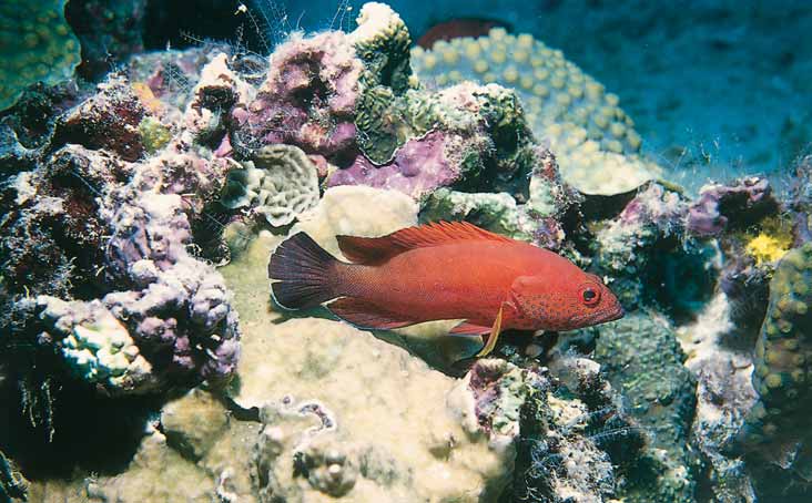
5
SUBTIDAL HABITATS
5.1 INTRODUCTION
This chapter describes methods for the survey of benthic
habitats and communities on both soft sediments (also termed
unconsolidated substrates) and hard substrates, but specifically
excludes seagrasses and coral reefs, which are dealt with in
detail elsewhere in this guide.
These methodologies are largely based upon, or adapted
from, ENGLISH et al. (1997). However, it is notable that ENGLISH
et al. do not specifically address the survey of any subtidal hard
substrates except for coral reefs. The survey methods for hard
substrates presented here are adapted from a number of sources,
including the coral reef survey methods of ENGLISH et al. (1997),
survey methods used by SHEPPARD & SALM (1988) for coral
communities in Oman, and those of DEVANTIER et al. (1998) for
coral reefs in the western Pacific.
5.2 GENERAL PRINCIPLES
The methods utilised for these two types of benthic habitat
are very different, with those for soft sediments generally being
carried out remotely using dredges and grabs, and those for hard
125

---

Standard Survey Methods
substrates being carried out by divers using
natural impacts over time. Monitoring surveys
scuba gear or, occasionally, snorkelling
will frequently require a more spatially
equipment. General methods common to all
intensive sampling regime within the survey
subtidal surveys are considered below,
areas, and greater replication of samples
whereas methods specific to either hard or
within sites, than baseline surveys.
soft substrate sites are dealt with separately at
a later stage in this chapter.
5.2.3 Temporal variation
The first step in any survey programme is
Temporal variation in natural
a clear understanding of the objectives, as
communities should always be taken into
these will frequently determine aspects of the
account in both design of surveys and
design of the survey, from large-scale
interpretation of results. The effects of
considerations of site selection to details of
seasonality vary greatly throughout the
equipment to be used.
PERSGA region (see for instance SHEPPARD et
al. 1992, pp. 121­140). The magnitude of
seasonal effects in the northern Red Sea is
5.2.1 Baseline surveys
minimal in comparison to those found in the
monsoon upwelling areas of the eastern Gulf
All subtidal sampling programmes, and
of Aden, but may nevertheless contribute
particularly those utilised for long-term
significantly to natural variation in sampling
monitoring programmes, require a knowledge
results.
of both the spatial and temporal variability of
the communities under study. There is a
general lack of detailed understanding of such
5.2.4 Pre-survey information search
variability in tropical soft-bottom
communities and also in tropical non-coral
When planning surveys, a search for
reef hard substrates. Consequently, there is a
relevant information already in existence
need for baseline surveys of such habitats to
should be carried out. This may provide
provide an understanding of broad-scale
valuable background information related to
variability in the survey area. Such baseline
areas to be surveyed, and in some cases also
surveys should provide information about
historical detail of direct relevance. Potential
variability within and between different types
sources to be researched include:
of habitats (e.g. gravel, sand and fine sediment
for soft bottom communities, or horizontal
Published scientific literature,
and vertical surfaces on hard substrates) and
across environmental gradients such as depth.
Consultancy reports and other `grey'
literature,
Maps, nautical charts and aerial
5.2.2 Monitoring surveys
photographs.
Having carried out baseline surveys to
characterise the broad habitat and community
Of these, the existence and location of
types within an area, and to establish the
relevant maps, charts and scientific literature
nature and degree of biological variability,
is relatively straightforward to establish. In
repeated surveys of the same sites within the
contrast `grey'
literature and aerial
area will provide information that can be used
photographs can be very difficult to identify
to monitor the effects of anthropogenic or
and locate, largely because the distribution of
126

---

Subtidal Habitats
such information is frequently limited or
required as in the case of monitoring
restricted and there are few or no central
surveys that need frequent re-
information sources related to them.
sampling. (To reduce the chance of
losing the buoy, it may be necessary to
secure it slightly below the surface).
5.3 STANDARD METHODS FOR
Describing the areas in relation to
ALL SURVEY OR SAMPLING
readily visible distinctive features.
SITES
This may be best achieved by the use
of a hand-drawn and annotated map or
diagram1.
5.3.1 Recording site location
It is essential to record the locations of all
survey and sampling sites accurately. The
By its nature, a lat/long position records a
preferred basis for recording site location is
point location. The linear nature of transects
latitude and longitude (hereafter referred to as
and sledge tows means that recording of such
lat/long). The existence of an accurate and
survey sites requires additional information:
precise lat/long is essential for:
Record two lat/long positions, one at
Mapping of sites and data, whether
the start of the transect or tow and one
onto hard-copy maps or into
at the end.
computer-based Geographical
Record the length and/or duration of
Information Systems (GIS),
transect/tow (usually recorded as
Enabling repeated surveys of the same
duration and, if a tow, speed).
site. This is particularly essential for
Record the direction of transect/tow (a
monitoring.
compass bearing, or a descriptive
account such as `parallel to the shore'
or `along the depth contour').
Hand-held Global Positioning Systems
(GPS)
Ideally any field surveyor or survey team
If a GPS is not available
should have access to a hand-held Global
If a GPS is not available, it is still possible
Positioning System (GPS). These pieces of
to record site location in inshore areas
equipment are increasingly robust, accurate and
precisely enough to enable accurate mapping
reliable and provide a lat/long accurate to within
and subsequent return to the site, if sufficient
100 m or less. If a greater degree of precision is
care is taken. This can be done by measuring
required than can be provided by a GPS then,
and recording compass bearings to at least
once the site has been located by GPS, further
three prominent landmarks, to provide
precision can be achieved either by:
triangulation. The position of each site should
then be mapped onto large-scale maps or
Marking the exact position of the
navigation charts and the lat/long calculated
survey/sampling site with a buoy;
as precisely as possible from the map or chart.
useful when return to the site is
This method is more time-consuming and
1 Ensure that the features used in any such description are not of a type that may change position or disappear between
surveys! For example, "Where the paved road ends and the dirt track begins" will not be useful if the paved road is
subsequently extended. The same is true of "...exactly 30 m offshore from the high tide mark, directly south of the parked
bulldozer" when the bulldozer may be driven away. (Both of these are genuine examples from survey record forms.)
127

---

Standard Survey Methods
generally less accurate than using a GPS,
Depth sounder or weighted shot line
which remains the preferred method. If a GPS
for measuring depth. Option: where
subsequently becomes available then sites
diving is being carried out as part of
should be re-visited to record their positions.
the survey, the depth gauge of a dive
computer is the preferred method for
determining depth of sample site.
5.3.2 Recording ambient environmental
Secchi disc for measurement of
parameters
visibility (except at very turbid sites,
Ambient environmental parameters
this is only relevant to deeper sites).
describing prevailing conditions at a survey
site should generally be recorded when a
Specialist equipment (not always
survey is carried out or samples taken. This is
available)
particularly the case for monitoring surveys,
Portable oxygen meter (splash-proof if
where ambient conditions may need to be
possible!)
taken into account in the interpretation of
results.
Remote water sampling bottles (e.g.
Nansen bottles, Figure 5.1).
Recording of many of these ambient
parameters can in practice be impractical or
Procedures
impossible for a number of reasons, such as a
Record the depth at the survey site
lack of appropriate specialist equipment (e.g.
either by depth sounder if available, or
oxygen meters, remote water sampling
by weighted graduated line if not (if
bottles) or a lack of opportunity (e.g. time of
currents are present which pull the line
day and light requirements for Secchi disc).
to one side, so giving an over-
The most important parameter, depth, is
estimation of depth, record this fact on
fortunately almost invariably straightforward
the survey data form). At sites
to measure and can be done without any
surveyed by divers, a diver's depth
specialist equipment. Other parameters should
gauge or dive computer can be used.
be measured when equipment and opportunity
Note however that gauges or
allow. When long-term environmental
computers showing depth with a
monitoring is to be carried out, then
resolution of 10­15 cm (4­6 inches)
investment of resources in the purchase and
are preferred, particularly at shallower
use of the relevant specialist equipment
sites.
becomes both more practical and more
necessary.
Read the water temperature 30 cm
below the surface before sampling
begins (this is the `surface' water
Equipment
temperature).
Thermometer accurate to +/­ 0.5°C for
Use a small screw-topped bottle to
measurement of surface water
collect a sample of water from 30 cm
temperature.
below the surface for salinity
Refractometer for salinity measurements
measurement using the refractometer.
and small plastic bottles for sampling of
For surveys where diving is to be
water at the surface (and at sampling
carried out the sample should be
depth, if diving is being carried out).
collected from the survey depth at the
time of the survey, by one of the divers
128

---

Subtidal Habitats
carrying out the survey. Salinity
can be lowered on a line and closed
measurements are particularly
remotely when they reach the required
important in any area where
depth. If these or similar devices are
freshwater input may be having an
not available then these measurements
impact, or where evaporation in
cannot be taken.
shallow semi-enclosed areas such as
lagoons may increase salinity
significantly.
5.4 SURVEY OF BENTHIC
Measure the turbidity at the site with
COMMUNITIES OF SOFT
the use of a Secchi disc. This should be
SEDIMENTS
carried out within two hours of
midday, with a cloudless sky. This
requirement means that recording
5.4.1 Introduction
turbidity can be impractical or
impossible to do at all survey sites.
Soft bottom habitats exist throughout the
At soft-bottom sites, a sample of
PERSGA
region, frequently closely
sediment should be collected by grab
associated with coral reefs or rocky habitats.
for grain size measurement at each
As well as supporting diverse and distinctive
sampling site. This sample should be
benthic and epibenthic communities, such
from the top 1­2 cm of the sediment,
areas of unconsolidated sediments form an
rather than from a cross-section of
integral part of both local and broader
different depths within the sediment.
ecosystems wherever they occur. Surveys of
the fauna of soft sediment habitats are
When a portable oxygen meter is
principally carried out for monitoring of
available dissolved oxygen
environmental impacts and pollution, for
concentration should be measured.
which they can be a powerful tool.
This parameter is of particular
importance when surveying areas
where organic enrichment or pollution
Although the biological survey of soft-
may be present. Water should be
bottom habitats has been widely utilised for
collected from the surface and, when
environmental monitoring in cold and
possible, the sample depth. Oxygen
temperate regions, it is relatively under-
concentration should be measured
utilised in tropical regions (ALONGI 1990).
immediately after the water sample is
Extensive and rapid coastal development and
collected, minimising time for changes
the occurrence of commercial benthic trawl
in temperature, exposure to air etc. to
fisheries throughout large parts of the region
alter the oxygen concentration in the
mean that there is an increasing need for
water.
monitoring of soft bottom fauna throughout
the Red Sea and Gulf of Aden.
If diving surveys are carried out,
divers should use small plastic sample
bottles to collect water samples for
Two methods for quantitative or semi-
salinity or oxygen measurements at
quantitative sampling of soft bottom
the survey depth. When carrying out
communities are described here: grabs and
grab or dredge sampling this can only
sledges. These are both remote methods in
be carried out using remote sampling
which the sampling is carried out from boats.
devices such as Nansen bottles, which
129

---

Standard Survey Methods
Sledges provide semi-quantitative and
For grab samples: A hopper-type base
descriptive information about benthic
for secure emptying of grab samples
communities, while grabs provide more
and a winch (motor-driven or manual),
quantitative sample data. Each of these two
to raise and lower the grab
methods samples a different aspect of the
benthic community and, if possible, an
For sledge samples: a sorting box
assessment of soft-bottom benthic
(wood, plastic or metal, large enough
communities should include both sampling
to accommodate the entire width of the
methods. If this is not possible, then the use of
sledge's open end).
one of these methods will still provide
valuable information.
If washing/sieving is to be carried out on
board the boat:
Both methods require the use of motorised
Buckets or a seawater pump for
boats and specialist sampling equipment.
washing of samples
When the equipment is available they are
straightforward to carry out, the equipment is
Sieves (5, 2, 1, and 0.5 mm mesh
robust and its maintenance is simple.
sizes)
10% formalin and 70% alcohol
Both of these remote survey methods are
Containers for samples
destructive to varying extents and, as a result,
may be unsuitable for use in certain locations
Sample/site recording sheets
(such as marine protected areas). The sledge
in particular, which is towed behind a boat
Sample labels and pencils.
and impacts considerably larger areas of sea
floor than the grab, is unsuitable for surveys
of areas where communities of long-lived and
Equipment for sorting of samples in the
fragile benthic organisms are known to occur
laboratory:
such as hard and soft corals, whip corals and
other large invertebrates. This is particularly
Sorting trays
the case for monitoring surveys, where
repeated sampling is necessary. In such cases
Petri dishes or similar small sorting
a decision must be made about the costs and
containers
benefits of carrying out sledge surveys, on a
case-by-case basis.
Binocular microscope
Forceps
Equipment needed
Containers for storage of sorted
Equipment for fieldwork:
samples.
Motorised boat
5.4.2 The Grab
GPS and/or compass
Target groups: non-mobile epifauna and
shallow infauna; principally used for
Sample gear (sledge and/or grab)
biological monitoring surveys (e.g. van Veen
grab, Figures 5.2 and 5.3).
130

---

Subtidal Habitats
Advantages
Label samples clearly with date, site,
Quantitative sampling, particularly
sample number and replicate number
useful for monitoring programmes
as soon as they are removed from the
grab and placed into any other
Relatively easy to use from a boat.
container. This information should be
written in pencil on waterproof paper
and placed inside the sample container
Disadvantages
(if waterproof paper is not available,
Can be difficult to use reliably in areas
thin card or strong ordinary paper can
of coarse sediments, particularly those
be used instead). The date, sample and
with large pebbles or rubble.
replicate number should also be
written in permanent marker on the
outside of the sample container.
Procedures
Ensure that this is done in a place
Grab samples for general
where the chances of the writing being
characterisation are taken at regular
rubbed off are minimal, such as on the
intervals along transects running at
lid.
right angles to the shore.
Sieve the sample through the set of
For examination of the effects of
sieves, discarding run-off water and
specific point sources of impact, such
silt. (Use of a 0.5 mm sieve may
as effluent outfalls, a grid is used to
prove impractical due to clogging. If
locate sampling points all around the
this is the case it is acceptable not to
source of the potential impact.
use this smallest sieve size, so long as
Sampling may be more concentrated
the method used is consistent
in the immediate vicinity of such an
throughout each survey, and between
impact.
all surveys which may be compared
with each other.)
A minimum of three grab samples
should be taken at each station. If time
Preserve echinoderms, soft corals and
and other resources permit (both in the
sponges in 70% or 100% alcohol
field and for subsequent laboratory
(100% for crinoids, brittlestars and sea
sorting, bearing in mind that sorting
cucumbers; then transfer to 70% once
can be extremely time-consuming) the
initial preservation is completed).
preferred sample size is five grab
Preserve all other material in 10%
samples per station.
formalin for initial preservation.
Formalin concentration can
Samples can be sieved on board the
subsequently be lowered to 5% or 4%.
boat or after return to the shore. If not
A cut should be made in the body
sieved immediately samples should be
walls of large organisms such as sea
stored in seawater in the interim, in
cucumbers to allow entry of
sealable buckets. It is essential that
preservative to the body cavity. All
samples are sieved and placed in
preservation and sample storage
preservative on the same day that the
should be in wide-mouthed airtight
sampling takes place. Store samples
containers, preferably made of plastic
out of direct sunshine until sieved, to
for safety.
prevent overheating.
131

---

Standard Survey Methods
5.4.3 The Sledge
and the amount of time and other
resources available. Larger areas will
Target groups: benthic epifauna;
generally be sampled at wider
principally used for baseline surveys and
intervals. If the survey is designed to
monitoring surveys (e.g. the Ockelmann
examine the impact of a site-specific
sledge, Figure 5.4).
activity then transects, and tows across
transects, may be closer together
nearer to the point of the impact.
Advantages
Samples a different component of the
Carry out three replicate tows at each
benthic fauna from a grab, so provides
site.
a complementary data set.
Speed and duration of all tows should
A
good method for initial
be consistent (nominally about 2
characterisation of an area.
knots, equivalent to a walking pace,
and for 5 or 10 minutes).
Relatively large area of sea floor
sampled means the dredge is more
After completion of the tow retrieve
likely than a grab to provide a
the sledge and empty the contents into
description of a site including locally
sieves placed on top of a sorting tray
rare taxa.
or box. Rinse with seawater to remove
fine silt and place all specimens into
sample containers with preservative.
Disadvantages
Larger specimens can be removed
Can be unacceptably destructive if
from the sieves and placed into
used in areas dominated by large and
separate containers.
long-lived invertebrates and is thus
inappropriate for repeated sampling
Label samples clearly with date, site
and monitoring programmes in certain
number, sample number and replicate
areas.
number as soon as they are removed
from the sledge and placed into any
Only provides semi-quantitative or
other container. This information
descriptive data about a site.
should be recorded both inside and
outside the sample container in the
Being towed, the sledge can become
manner described previously for grab
caught on obstructions on the sea
samples.
floor.
Sample specimens should be
Procedures
preserved in 70% or 100% alcohol, or
Tows for sledge surveys are carried
in formalin, in the manner described
out at regularly spaced intervals across
previously for grab samples.
a transect. The transect itself will
usually be at right angles to the
shoreline and so tows will be parallel
to the shore. Transects are spaced
along the shore at intervals determined
by the size of the area to be surveyed
132

---

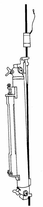
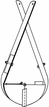
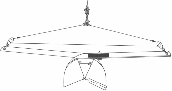
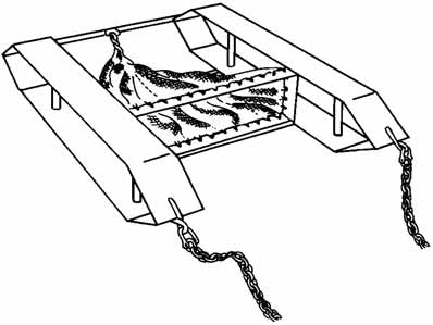
Subtidal Habitats
Figure 5.1 Nansen bottle
Figure 5.2 van Veen grab, closed
Figure 5.3 van Veen grab open
Figures adapted from ENGLISH et al. 1997.
Figure 5.4 Ockelmann sledge
133

---

Standard Survey Methods
5.4.4 Sorting of samples collected by
Data are recorded as counts for all
grab or sledge
organisms except colonial organisms
such as corals, sponges and coralline
algae. For these record wet weight for
Samples collected by either of the above
each family or species. For non-
methods should be sorted in a laboratory. It is
coralline algae also record wet weight
essential to minimise exposure of personnel to
of each species or group.
the fumes of preservatives, so those
preservatives should be removed as far as
Data are stored in hard copy on
possible before sorting is carried out. To do
standard sample record sheets, which
this:
include all data on site number, sample
number, date of collection, etc. Where
Pour off excess preservative through a
possible data are also entered into a
fine-mesh sieve (as far as possible
computer database for storage. Use of
recycle all preservatives). In the case
a database such as MICROSOFT ACCESS,
of formalin it is essential to dispose of
which is compatible with programmes
any unwanted excess or waste safely.
to be used for analysis, such as EXCEL
Do not simply pour down the drain.
or SPSS, is recommended.
Thoroughly rinse the sample in clean
Do not discard samples after sorting.
fresh water or seawater to remove as
Instead store in formalin or alcohol,
much preservative from the sample as
labelled with sample details on paper
possible.
inside the airtight sample container
Carry out sorting where there is a good
and with permanent marker on the
circulation of air. The use of a fume
outside. If storage space is available it
hood for sorting is preferred, if one is
is recommended that samples be
available.
retained for at least two years in case
re-examination is needed.
Once preservatives have been removed:
5.4.5 Data analysis for grab and sledge
Carry out gross-level sorting of
samples
samples in large plastic sample trays
(preferably white) under good
A good summary of the communities
lighting. Remove larger specimens at
within samples can be provided by simple
this stage.
descriptive analyses of data, including:
Place sub-samples from material
Species lists
remaining in the trays into petri dishes,
and sort into major classes under a
Densities of species/families
binocular microscope.
Distributions of species/families (best
Subsequently sort to at least family
represented as a map or schematic
level using taxonomic keys. (Sorting
diagram).
to species level is a time-consuming
task. While sample sorting and
For examination of relationships between
identification should be carried out to
variables, both biological and environmental,
species level if possible, where it is not
simple correlations and regressions should be
possible sorting to family level is
acceptable.)
134

---

Subtidal Habitats
used. If in any doubt about whether there is a
Multivariate analyses require specialist
causal relationship, then correlations should
computer programmes, but they are powerful
be used.
tools for revealing patterns in biological
communities, and are commonly used to
explore data sets, and to reveal similarities
Diversity indices usefully summarise
and differences between different sites, or
abundance data sets of species, and of higher
changes within a site over time. A number of
taxa such as families, to provide a single
software packages have been developed that
number representing a measure of diversity in
aid the application of multivariate analyses to
a sample or at a site (see MAGURRAN 1988 for
environmental data, including some
a comprehensive review of ecological
specifically designed for application to the
diversity measures).
study, survey and monitoring of marine
ecosystems.
Two components of diversity are species
richness (number of species) and species
When appropriate software is available,
evenness (how equally abundant the species
cluster analyses and multi-dimensional
found in the sample are). In general, if a
scaling (MDS) analysis should be used to
sample is heavily dominated numerically by
identify patterns of similarity and difference
one, or a few, species it will be less diverse
between samples and sites. The nature of
than one in which abundances are more
those similarities and differences can then be
evenly spread between species. An
examined in more detail if necessary.
abundance of diversity indices exists; these
principally vary in how much weighting they
give to one or other of these aspects of
5.4.6 Data presentation
diversity.
Presentation of data about abundance,
density, diversity and ambient parameters can
One of the most commonly used
be done in both tabular and graphical form
measures of diversity in marine surveys and
and will provide a useful description of the
monitoring is the Shannon-Weiner index
sampled communities:
(H), also known as the Shannon index. This
index is dependent upon both the species
Tables should be used where
richness of a sample and the evenness and so
presentation of exact data values is
provides a useful combination of the two
required. This is frequently in addition
types of measure.
to graphical representations.
Graphical representation is
The Shannon-Weiner index (H):
particularly useful for presentation of
descriptive parameters, such as
differences between sites, or
H = s pi(log 2 pi)
differences between different surveys
i=1
of the same site. Both direct values,
where pi is the proportion of the ith species
such as abundances, and derived
(or other taxon such as genus or family) in the
values, such as diversity indices, can
sample.
be plotted graphically.
135

---

Standard Survey Methods
Multivariate analyses are generally
rocky substrates with a variable
presented in formats specific to the analysis
cover of living coral, sometimes
carried out (dendrograms, MDS plots, etc).
including more or less well-
developed coral reefs.
Representation of data through plotting
(both characteristic of the Gulf of
onto maps can be an invaluable aid to both
Aden and Arabian Sea).
understanding and to decision making. A
computer-based GIS is the preferred method
Within the PERSGA region, non-coral
for mapping (e.g. ARCINFO, or the PC-based
reef hard substrate habitats are largely
ARCVIEW). In the absence of GIS facilities,
confined to the Gulf of Aden including the
use of hard copy maps with different overlays
Socotra Islands, and to the Arabian Sea coast
illustrating different parameters can also be
of eastern Yemen. Here, non-coral hard
valuable and productive.
substrates can be extensive wherever rocky
shores occur and at offshore reefs, frequently
forming a patchwork with areas of relatively
high coral cover. (The term `reefs' is used here
5.5 NON­CORAL REEF HARD
to mean any area of raised hard substrate,
SUBSTRATE COMMUNITIES
whether composed either of corals or non-
biogenic rock).
5.5.1 Introduction
Globally, the study of the ecology and
The PERSGA region is one of the most
diversity of non-coral tropical reefs and hard
ecologically variable areas of the tropical
substrates in category 3, above, is
Indo-west Pacific. This naturally occurring
comparatively neglected. Studies in the
variability in shallow subtidal habitats
northern Indian Ocean and Arabian region
manifests itself most conspicuously on hard
have been carried out in Oman and Sri Lanka
substrates. Hard substrates within any large
(e.g. SHEPPARD & SALM 1988; GLYNN 1993;
area of the PERSGA region may be
RAJASURIYA et al. 1998). These studies,
dominated by:
however, have concentrated to a greater or
lesser extent on the coral communities that are
1. Well-developed coral reefs
present, even at extremely low densities, on
(characteristic of most of the northern
virtually all hard substrates in the region.
and central Red Sea), or
Consequently the non-coral component of
such communities is relatively poorly studied
2. A combination of coral and algal reefs
(the exceptions to this are macroalgal
(characteristic of much of the southern
communities, which have been extensively
Red Sea) or
studied in some areas).
3. A frequently very patchy combination
of:
Among the first to address this
rocky substrates with little or no
combination of different coral and non-coral
living coral (but often with high
hard substrates in the Arabian region were
diversity of other benthic
SHEPPARD & SALM (1988) in their study of the
organisms, including both
corals of Oman. Being principally a study of
invertebrates and seaweeds),
coral communities, they did not address in any
detail the wider nature of communities living
136

---

Subtidal Habitats
on non-coral hard substrates, but the paper does
5.5.2 Methods
provide a useful basis for differentiating broad
types of benthic hard substrate community
The methods described here are
found in the region. This differentiation is
principally based upon or adapted from those
based on how dominant hard corals are at a site
of ENGLISH et al. (1997), SHEPPARD & SALM
and how well developed coral reef structures
(1988) and DEVANTIER et al. (1998).
are. The categories SHEPPARD & SALM (1988)
identified on this basis are as follows.
For broad habitat characterisation surveys,
and surveys which will not be used for
Category A
monitoring purposes and so will not require
Clear coral reef growth exists, where the
return visits to exact locations, transects need
bedrock is overlaid or obscured by the
not be marked permanently. If return to the
characteristic reef topography of a horizontal
exact place is required then the locations of
reef flat and a reef slope.
survey sites must be marked in a manner that
enables return to and re-survey of the exact
site.
Category B
Coral framework is present in which
corals provide a substrate cover of > 25%,
As a general rule, for surveys carried out
and sometimes exceed 75%, but there is no
by divers the number of different workers
reef topography. Instead gross substrate
recording data should be kept to a minimum,
topography and slope remains unchanged
both within one survey and for repeat surveys
compared to adjacent coast not colonised by
of the same areas, in order to reduce between-
coral.
observer error.
Category C
Procedures
Coral cover is < 15%, or too low to be
Prior to carrying out any survey
considered as providing framework. Corals
transects, a rapid assessment of the site
remain diverse but do not include more than
is carried out to enable the site to be
scattered colonies of the main framework
assigned to one of categories A, B or C
builders. All colonies are attached directly
as defined by SHEPPARD & SALM
onto bedrock.
(1988). This assessment can usually be
carried out without the use of scuba
equipment. In most of the Red Sea this
This section deals with hard substrate
step may be unnecessary, as almost all
communities of type C. Types A and B are
shallow hard substrates here fall into
covered in the chapter which describes survey
Category A.
methods for coral and coral communities.
Although categories B and C could
For sites in categories A or B survey
theoretically grade into each other, in practice
methods described in the chapter on
values for living coral cover tend to be widely
corals and coral communities should
separated into these two groups. Also see
be used.
chapter on seagrasses and seaweeds for
At sites falling into category C, a
survey methods to be used specifically to
range of standardised depths is
provide descriptions of macroalgal
surveyed. If hard substrates are limited
communities.
to shallow depths, then transects are
137

---

Standard Survey Methods
only carried out to the greatest
Make a note of all observations of
standardised depth at which hard
human utilisation and impacts at the
substrates occur. Standard depths are:
site (e.g. fishing activity, litter, fish
traps, lost nets, anchor damage, etc.).
1­2 m (snorkelled)
Data are stored in hard copy on
7 m
standard sample record sheets, which
15 m
include all data on site number, sample
number, date of collection, etc. Where
Record the approximate mean depth
possible, data are also entered into a
along the transect at which hard
computer database for storage. Use of
substrates are replaced by
a database such as MICROSOFT ACCESS,
unconsolidated substrates.
which is compatible with programmes
to be used for analysis, such as EXCEL
Transects are standardised at 100 m
or SPSS, is recommended.
long (equivalent to a 10 minute slow
swim) and a nominal 4 m wide
(estimated by eye, 2 m either side of
5.5.3 Data analysis
the central line of the transect).
Graphical representations of both
The percentage cover of each of eight
substrate and taxonomic categories provide
substrate categories and eight
useful descriptive summaries and exploratory
ecological categories (Table 5.1) are
analysis of survey data.
estimated by eye using categories of
percentage cover (Table 5.2). Data are
recorded onto prepared recording
When appropriate computer software is
sheets if waterproof paper is available,
available, multivariate analyses are used to
or directly onto underwater slates.
group transects and sites on the basis of the
eight substrate variables recorded to provide
The abundances of each of 20
general site descriptions. Finer resolution is
taxonomic categories (Table 5.3) are
obtained through carrying out similar analyses
recorded using abundance categories
on the taxonomic data. The nature of the
(Table 5.2).
similarities and differences between groups of
Record all observed occurrences of
sites, and between times, can then be
coral disease, bleaching, crown-of-
examined in more detail if necessary.
thorns starfish, Drupella, or high
concentrations of sea urchins. When
occurring within transects record the
The groupings identified by multivariate
approximate percentage of coral
analyses can be used to map distribution of
colonies affected, or the numbers of
habitat and broad community types.
starfish or urchins observed. Outside
the transect record presence or
absence. Note that crown-of-thorns
starfish may occur even in areas of
extremely low coral cover and may
feed on soft as well as hard corals.
138

---

Subtidal Habitats
5.5.4 Data presentation
Multivariate analyses are presented in
formats specific to the analysis carried out
Presentation of data about abundance,
(dendrograms, non-scalar plots, etc.).
diversity and ambient parameters can be done
in tabular or graphical form.
Representation of data through plotting
onto maps can be an invaluable aid to both
Graphical representation is particularly
understanding and to decision making. A
useful for presentation of descriptive
computer-based GIS is the preferred method
parameters, such as differences between sites,
for mapping (e.g. ARCINFO, or the PC-based
or differences between different surveys of the
ARCVIEW). In the absence of GIS facilities,
same site. Both direct values such as
use of hard copy maps with different overlays
abundances, and derived values such as
illustrating different parameters can be
diversity measures, can be plotted graphically.
valuable and productive.
Tables should be used where presentation
of exact data values is required.
Substrate category
Ecological category
Rock (modern biogenic)
Hard coral (live)
Rock (non-biogenic or fossil)
Hard coral (dead)
Large blocks
Soft coral
Small blocks
Turf algae
Rubble (non-biogenic)
Kelps (Sargassum spp. etc.)
Rubble (coral)
Other macroalgae
Sand/gravel
Coralline algae
Silt/mud
Other invertebrates

Table 5.1 Substrate categories for hard substrate surveys.

Category %
cover
Abundance
(substrate)
(taxonomic)
0 Absent
Absent
1
>0 ­ 10
Rare
2
11 ­ 30
Uncommon
3
31 ­ 50
Common
4
51 ­ 75
Abundant
5
75 ­ 100
Dominant

Table 5.2 Percentage cover and abundance categories for hard substrate rapid assessment surveys.
139

---

Standard Survey Methods

Substrate category
Category
Description.

Hard corals.
Acropora

Pocillopora

Branching ­ other
All other branching growth forms.
Massive
Massive corals (except Porites).
Porites
All Porites colonies.
Encrusting

Other hard corals
All living hard corals not falling into

the above categories.
Millepora

Hard coral - dead
All in situ dead hard corals.
Hard coral - rubble
All displaced or broken fragments of
dead hard coral.
Soft corals,
Xeniidae

gorgonians, etc.
Other soft corals
All other soft corals
Gorgonians
Gorgonians, sea whips and black
coral
Others. Corallimorpharians

Other sessile invertebrates

Calcareous algae

Turf algae

Algal assemblage/mat
Multi-species areas of small
Phaeophytes
algae/mat
Other macroalgae
Kelps (Sargassum spp. etc.)
All other macroalgae

Table 5.3 Taxonomic categories for hard substrate surveys.
140

---

Subtidal Habitats
5.6 REFERENCES
SHEPPARD, C.R.C. & SALM, R.V. 1988. Reef
and coral communities of Oman, with a
description of a new coral species (Order
Scleractinia, genus Acanthastrea). Journal of.
ALONGI, D.M. 1990. The ecology of tropical
Natural History 22: 263­279.
soft-bottom benthic ecosystems. Oceanography
and Marine Biology Annual Review 28:
381­496.
Other Recommended Literature
CLARKE, K.R. & WARWICK, R.M. 1994.
DEVANTIER, L.M., DE'ATH, G., DONE, T.J. &
Change in Marine Communities: An Approach
TURAK, E. 1998. Ecological assessment of a
to Statistical Analysis and Interpretation.
complex natural system: A case study from
Plymouth Marine Laboratory, UK.
the Great Barrier Reef. Ecological
Applications 8 (2): 480­496.
FISCHELSON, L. 1971. Ecology and
distribution of the benthic fauna in the
shallow water of the Red Sea. Marine Biology
ENGLISH, S., WILKINSON, C. & BAKER, V.
10: 113­133.
1997. Survey Manual for Tropical Marine
Resources. 2nd Edition. Australian Institute of
HOLMES, N.A. & MCINTYRE, A.D. 1984.
Marine Sciences. 390 pp.
Methods for the Study of Marine Benthos.
Blackwell Scientific Publications, London.
387 pp.
GLYNN, P.W. 1993. Monsoonal upwelling and
episodic Acanthaster predation as probable
MASTALLER, M. 1978. The marine molluscan
controls of coral reef distribution and
assemblages of Port Sudan, Red Sea.
community structure in Oman, Indian Ocean.
Zoologische Mededelingen 53: 117­144.
Atoll Research Bulletin 379: 1­66.
OCKELMANN, K.W. 1964. An improved
detritus-sledge for collecting meiobenthos.
MAGURRAN, A.E. 1988. Ecological Diversity
Ophelia 1: 217­222.
and its Measurement. Princeton University
Press. 179 pp.
PRICE, A.R.G., CROSSLAND, C.J., DAWSON
SHEPHERD, A.R., MCDOWALL, R.J., MEDLEY,
P.A.H., ORMOND, R.F.G., STAFFORD-SMITH,
RAJASURIYA, A., ÖHMAN, M.C. & JOHNSTONE,
M.G. & WRATHALL, T.J. 1988. Aspects of
R.W. 1998. Coral and sandstone reef-habitats
seagrass ecology along the western shore of
in north-western Sri Lanka: patterns in the
the Red Sea. Botanica Marina 31: 83­92.
distribution of coral communities.
Hydrobiologia 362: 31­43.
WAHBEH, M.I. 1981. Distribution, biomass,
biometry and some associated fauna of the
seagrass community in the Jordan Gulf of
SHEPPARD, C.R.C., PRICE, A.R.G. & ROBERTS,
C.M. 1992. Marine Ecology of the Arabian
Aqaba. Proceedings of the 4th International
Region: Patterns and Processes in Extreme
Coral Reef Symposium 2: 453­459.
Tropical Environments. Academic Press.
359 pp.
141

---

Standard Survey Methods
142

---

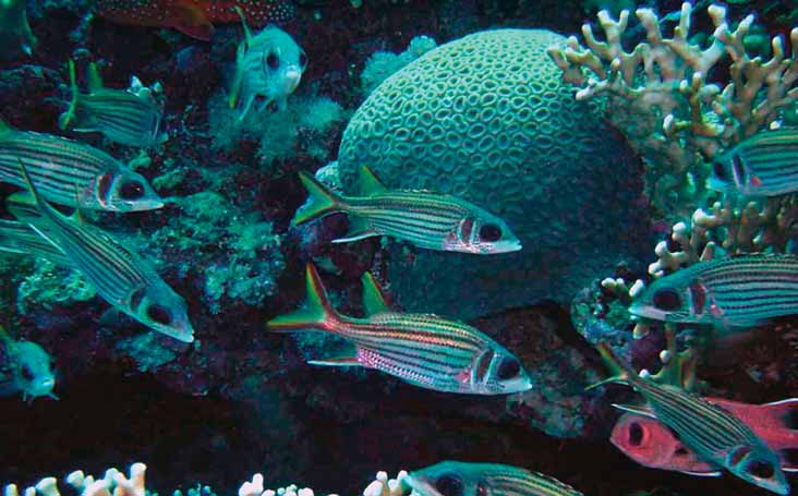
6
REEF FISH
6.1 INTRODUCTION
Fishes are the most conspicuous inhabitants of coral reefs,
occurring in schools of up to thousands of individuals and
displaying striking colours, shapes and patterns. Fishes not only
contribute to the aesthetic value of coral reefs, they also
constitute a major component of total biodiversity (BELLWOOD &
HUGHES 2001), are a source of economic value (RUSS 1991) and
contribute to the overall health and resilience of coral reef
ecosystems via a number of ecological processes (BELLWOOD et
al. 2003).
About 1,350 species of fishes are known from the Red Sea
(GOREN & DOR 1994). Distinct assemblages occur in the Gulf of
Suez, the Gulf of Aqaba and the central and northern Red Sea,
the southern Red Sea and the Gulf of Aden (SHEPPARD et al.
1992). The level of endemism amongst Red Sea fishes is about
17%. However, as SHEPPARD et al. (1992) point out, this average
value has a great range. For example, the degree of endemism
amongst small, benthic, territorial groups such as dottybacks
(Pseudochromidae) and triple fins (Trypterygiidae) is about
90%, while endemics are almost absent amongst pelagic species.
143

---

Standard Survey Methods
There are very few accounts of the
among reefs of the Farasan Islands (Saudi
ichthyofauna of the Gulf of Aden. AL-SAKAFF
Arabia) shared by a number of villages, was
& ESSEN (1999) listed 195 species of fishes
traditionally used as a means of preventing the
caught in commercial trawlers from the Gulf
over-exploitation of fish stocks on shared
of Aden and Arabian Sea coastline of Yemen.
reefs. However, the practice has broken down
KEMP (2000) surveyed the ichthyofauna of the
in the face of increased fishing pressure from
Shabwa and Hadramaut provinces of the
foreign workers who do not understand local
Republic of Yemen and recorded 267 species,
customs and have different economic needs
including eight new records. KEMP (1998)
(GLADSTONE 2000). The isolation of the
surveyed a number of reef-associated fish
Socotra Archipelago from markets, seasonal
groups in the Socotra Archipelago. Then,
weather that limits access to many reefs and a
using regional data on chaetodontid fishes,
cooperative, traditional management system
KEMP (1998) distinguished the Arabian
ensured that catches of fish and sharks were
representatives into three groups. These are
sustainable. However, increasing international
the Red Sea and western Gulf of Aden;
demand for shark fins and the high prices paid
Socotra, Oman and the Gulf; and east Africa,
for dried fins have caused this fishery to
the Seychelles and the Maldives. On this
become unsustainable (MACALISTER ELLIOTT
basis, the Socotra Archipelago has a
& PARTNERS 1996). In order to support
regionally high conservation value because its
sustainable uses, traditional fisheries
fish fauna appears to be distinctly different
management practices will need to be
from the rest of the Red Sea and Gulf of Aden.
supplemented by alternative approaches, such
as the establishment of marine protected
areas (MPAs).
The fishes of the Red Sea and Gulf of
Aden have been prominent in the recent
scientific history of the region, with many of
There are a number of pressures on the
the early European explorers undertaking
biodiversity and natural systems of the Red
ichthyological collections (VINE & SCHMID
Sea and Gulf of Aden arising from the rapid
1987). Artisanal fishing has been socially and
development and widening exploitation of the
economically important for centuries along
marine and coastal environments (PERSGA
the coastlines of all countries bordering the
1998; WILKINSON 2000). These pressures
Red Sea and Gulf of Aden. Low population
include disturbance to coastal wetlands,
densities, traditional management practices
clearing and degradation of mangroves, loss
and limited commercial demand have helped
of seagrass beds, destruction of coral reefs,
to keep this activity ecologically sustainable
unsustainable use of living marine resources
(GLADSTONE et al. 1999). However, a number
(for example, through overfishing and
of developments threaten this sustainability,
unregulated shark fishing), threats to
such as the use of more modern equipment,
important species (such as marine turtles,
the availability of ice, the participation of
marine mammals and seabirds), marine
foreign workers (especially in the Saudi
pollution, poor planning of the coastal zone,
Arabian Red Sea waters), government
discharge of effluents, dredging and filling of
support, the spread of illegal fishing
coastal habitats, and reduction of freshwater
(especially for shark fins), aquaculture and the
flows to the coastal zone.
rise of recreational fishing in some areas.
Such developments have led to the decline of
traditional community-based management
A number of management initiatives have
practices. For example, the practice of
been set up in the Red Sea and Gulf of Aden
cooperatively rotating fishing activities
region that will require regular monitoring to
144

---

Reef Fish
assess their effectiveness, including the Red
Logistical constraints in long-term
Sea and Gulf of Aden Regional Network of
monitoring programmes mean that sites may
Marine Protected Areas (PERSGA/GEF
only be sampled annually. This could lead to
2002). Monitoring of natural systems and
erroneous conclusions about long-term
species of interest will generate feedback to
temporal trends if potential sources of
managers on the outcomes of management
variation occurring at the time of sampling
strategies and provide fundamental
(for example, time of day, tidal cycle or
information on natural dynamics. The quality
season) are not understood and accounted for
of the monitoring information is crucially
in the sampling design. For example,
important for ecologically and socially
THOMPSON & MAPSTONE (2002) found that
sustainable management.
variation in the abundance of fishes from the
families Chaetodontidae, Lethrinidae and
Labridae between successive days was as
Monitoring programmes implemented at
great as, or similar to, the variation in
the scale of a country or region can be
abundance between successive years. This
expensive and logistically difficult to
variation makes it difficult to detect changes
implement. The monitoring methods must be
that may be occurring as a result of human
time and cost-effective, whilst fulfilling the
disturbance or management intervention.
information needs of managers and being
appropriate to the species of interest. Most
monitoring programmes for fishes are
A variety of survey methods are used
designed to encompass a number of species. It
around the world for research, monitoring and
is therefore important that the methodology
survey programmes by scientists, management
and design of the monitoring programme are
agencies and community groups. Regional and
appropriate for the biology of the species and
global assessments of the status of fishes on
the scales at which natural fluctuations occur.
coral reefs are likely to be limited by the
In particular, the following biological factors
quality of the information collected and the
are likely to be important considerations in
range of methods used. The approach taken in
designing surveys: (1) spatial and temporal
the Red Sea and Gulf of Aden has been to
patterns in the distribution of the species; (2)
develop standard methods that will allow
size and frequency of movements, particularly
comparisons and assessments among the
in relation to the size of sampling units; (3)
countries in the region.
spatial and temporal scales at which
abundance varies. Important methodological
considerations include the size and shape of
The standard survey methods for fishes
the sampling unit (such as the transect) and
presented here will be used to evaluate the
the ways in which the units are surveyed.
status of fish assemblages and individual
Optimal transect dimensions will be those
species of importance in the Red Sea and Gulf
that, based on the results of pilot studies,
of Aden region and to monitor the way both
reduce variability, increase precision and are
change through time. Monitoring will be
logistically feasible to implement. Further
carried out in order to understand the scale of
design factors that need to be addressed
natural variations and to evaluate the
include the number of replicate sampling units
effectiveness of management.
and their spatial and temporal deployment
(MAPSTONE
& AYLING
1998). These
considerations will be addressed in the
The methods that will be used here are
standard survey methods for reef fishes
underwater visual surveys. Forms of this
presented below.
technique are now routinely used to assess
145

---

Standard Survey Methods
fish biodiversity for long-term monitoring
6.2 METHODOLOGIES
and for assessing the effectiveness of
management. A considerable amount of
A number of different underwater visual
research has been undertaken into the
survey methods for reef fishes are illustrated
methodological aspects of underwater visual
here. They provide for rapid, broad-scale
surveys for fishes, with the goal of
assessments of reef fish status (the Reef Check
eliminating bias and improving accuracy and
surveys), detailed information on the population
precision (THOMPSON & MAPSTONE 1997,
structure of a large number of key species,
2002). The present chapter provides a review
biodiversity assessments of regional fish faunas
of a number of existing survey methods.
and assessments of the impacts of aquarium fish
These include a method appropriate for use
collecting. Choice of method will depend on the
by community dive groups (the Reef Check
reason that information is required, the use to
method), techniques for rapid assessment
which this information will be put and on
and also an in-depth analysis of a method
technical and logistical capabilities.
suitable for the collection of detailed
information on distribution, abundance and
length of fishes inhabiting coral reefs. A
6.2.1 Reef Check Surveys
number of other survey methods are also
reviewed and described, which may be
The Reef Check survey methodology is
suitable for other applications in the Red Sea
designed to provide a rapid, broad-scale
and Gulf of Aden region.
assessment of the distribution and abundance
An analysis of Reef Check data collected in more than 60 countries between 1997 and 2001 has provided a
snapshot of the current status of fishes on coral reefs and an indication of trends in the abundance of some key
species.
Data collected by Reef Check teams between 1997 and 2001 revealed:
No spiny lobster were recorded at 83% of reefs surveyed, indicating severe overfishing
A significant decline in the abundance of butterfly-fish
No grouper larger than 30 cm were recorded at 48% of reefs surveyed, indicating severe
overfishing
Four species of reef fish are believed to be in `critical condition': Nassau grouper (not recorded
from 82% of shallow Caribbean reefs surveyed); Barramundi cod (absent from 95% of Indo-
Pacific reefs); bumphead parrotfish (absent from 89% of Indo-Pacific reefs); and humphead
wrasse (absent from 88% of Indo-Pacific reefs)
parrotfish greater than 20 cm in length were not observed on 55% of reefs surveyed
The Reef Check surveys also revealed substantial differences between regions in the dominant
groups of fishes: fish belonging to the families Scaridae and Haemulidae were most abundant on
Atlantic reefs, and fish belonging to the families Chaetodontidae and Lutjanidae were most
abundant on Indo-Pacific reefs
Marine protected areas appear to be showing benefits for some species of fishes in developing
countries: five of the 10 indicator species are more abundant in marine protected areas than
comparable fished areas.
Source: HODGSON & LIEBLER (2002)
Table 6.1 Five years of Reef Check, 1997 to 2001.
146

---

Reef Fish
of a number of fish species known to be either
surveys use transects that follow a depth
indicators of reef health (for example
contour which runs parallel to the shore or
chaetodontids) or susceptible to the effects of
reef face, not perpendicular to the reef face or
fishing (for example serranids and scarids).
along a depth gradient. Two depths are
The Reef Check method has been widely
surveyed at each site: shallow (2­6 m) and
adopted by recreational dive groups in more
mid-depth (6­12 m), with depth based on
than 60 countries (HODGSON 2000; HODGSON
lowest low water.
& LIEBLER 2002), including Egypt, Jordan and
Yemen. It is a rapid approach to surveys of
reef fishes that can be undertaken with a
Methodology
minimum of training. The Reef Check
Four transects of 20 m are surveyed for
methodology is included here because of its
each depth and site, with transects laid along
value in obtaining broad-scale snapshots of
the depth contour. The surveys proceed in the
the status of reef fish, its potential to provide
following manner:
more frequent surveys of specific sites and
because of its role in engaging and educating
Transects are laid using a 100 m
the wider community. The Reef Check
fibreglass tape measure with 5 m
methodology has provided information on the
intervals between replicate 20 m
global status of coral reefs and trends in reef
transects.
status over recent years (see Table 6.1).
Survey teams wishing to undertake Reef
One pair of divers lays out the
Check surveys and participate in the
complete 100 m tape measure then
programme should contact the Reef Check
swims back along the tape ensuring
organisation (listed under Web Pages).
that it lies clearly along the reef.
In sites where the reef is not
The following description of the Reef
continuous (for example, reef slope
Check methodology has been adapted from
areas interspersed with sand or drop-
R
offs) 20 m tape measures are used to
EEF CHECK (2003).
mark out the individual 20 m sections
of the transect, each separated by at
Site Selection
least 5 m.
Reef Check surveys are undertaken at
The start and end of the transect are
sites representative of the range of human
marked with floats, and the position of
impact occurring in an area. They should
one of the floats is recorded on a chart
include a site that is pristine or shows few
or with Global Positioning System
signs of human impact, one experiencing
(GPS). This allows the site to be easily
moderate levels of human impact (for
located for subsequent surveys. In
example from fishing or pollution) and one
addition, the position of the site in
that is severely impacted by human usage.
relation to prominent landmarks is
The Reef Check team surveys the most
recorded as a backup in case of loss of
pristine site in the area when it is not possible
GPS data.
to survey more than one site.
Surveys of fish transects start no
earlier than 0900 hours.
Surveys are performed on the exposed or
seaward section of reefs, on reefs that contain
Divers wait for 15 minutes after the
reef crest and reef slope habitats. Reef Check
transects have been deployed and
checked, to allow time for fish that
147

---

Standard Survey Methods
Common Name
Family or Species
Grouper > 30 cm
Serranidae
Grunts / sweetlips / margates
Haemulidae
Butterfly-fish Chaetodontidae
Broomtail wrasse
Cheilinus lunulatus
Humphead wrasse
Cheilinus undulatus
Bumphead parrotfish
Bolbometopon muricatum
Parrotfish > 20 cm
Scaridae
Moray eel (any species)
Muraenidae
Table 6.2 Groups of reef fishes recommended for survey in the Red Sea under the Reef Check programme
(Reef Check 2003).
may have been disturbed by the divers
The abundance of all fish observed is
laying the transect to return to the area.
recorded regardless of size, apart from those
belonging to two families, the Serranidae
Fish are surveyed by one or both
(groupers) and the Scaridae (parrotfishes),
divers of the buddy pair. If both divers
where only those exceeding 30 cm and 20 cm
in the buddy pair are experienced fish
respectively are recorded (Table 6.2). The
observers they alternate in surveying
lengths of groupers are estimated and
fish along 5 m lengths of the transect.
recorded on the data sheet in the Comments
The fish observer swims along the
section. For these reasons fish observers need
transect about 1 m above the tape and
to be proficient in estimating two distances
records the abundance of all indicator
underwater, the 2.5 m belt on both sides of
species (Table 6.2) in an area 2.5 m
the tape measure and the minimum lengths of
from both sides of the tape measure
groupers and parrotfishes. Reef Check survey
and up to 5 m above the substratum.
teams carry a 2.5 m pole that is placed on the
When the 5 m distance along the tape
substrate and observed by divers at the
measure is reached the observer stops
beginning of the dive, so that divers become
swimming and, while waiting for 3
accustomed to the scale of this distance
minutes, records the abundance of all
underwater. In addition, survey teams
indicator species that come out of
familiarise themselves with the 20 and 30 cm
hiding. At the end of the 3 minutes the
lengths by carrying a number of sticks of
observer begins swimming along the
these lengths and familiarising themselves
next 5 m section of transect.
with the appearance of these lengths at the
start of each dive.
This process is repeated until the end
of the 20 m transect is reached. The
buddy pair then swims the 5 m along
Site Descriptions
the tape measure to the beginning of
The characteristics of all sites included in
the next fish transect (fish are not
the Reef Check survey are described to allow
counted in this 5 m interval).
linkages to be made between the status of
reefs and the status of the indicator species
The abundance of all indicator species
(see Appendix 6.7.1). The site description is
is recorded on a standard data sheet
conducted at the same time as the fish surveys
(Appendix 6.7.1).
by other team members.
148

---

Reef Fish
6.2.2 Rapid Visual Counts
therefore be subject to more sources of
variation that are not accounted for than more
Rapid visual counts are frequently
formalised transect surveys.
undertaken in situations where the time and
resources available to collect detailed
information (such as species level data) are
Rapid visual counts have been used in a
unavailable, where a large number of sites
number of different applications. To describe
have to be surveyed or when it is desirable to
patterns in the distribution and abundance of
collect information from the same site on a
coral reef fishes across different reef types,
range of biophysical parameters (such as a
WILLIAMS (1982) employed 45 minute swim
subset of species and substrate composition).
surveys by divers. The surveys were
They can be in the form of qualitative or semi-
performed on the outer reef slope by divers
quantitative surveys.
swimming in a zigzag pattern from the surface
to 13 m depth and recording fishes occurring
within 5 m either side. Swims covered
Rapid visual counts are performed by
approximately 150 m of reef front. RUSS
free-swimming divers surveying a search area
(1984a,b) surveyed richness and abundance of
that has not been determined using transects
herbivorous reef fishes on the Great Barrier
or tape measures. Divers swim over the reef
Reef using 30 minute swims, during which
for a specified period of time recording fish
fishes occurring within 5 m either side of the
species and their abundance. Rapid visual
observer were recorded. The abundance of
counts are useful over large sections of
each species was recorded on a log 3
coastline for recording reconnaissance-level
abundance scale. SYMS (1995) defined the
information or preliminary data prior to more
habitat characteristics of blennioid fishes with
detailed surveys (ORMOND et al. 1984). They
75 minute swims during which all
are also useful for trained observers for
occurrences of fishes were recorded and the
obtaining the same level of information (fish
habitat and micro-habitat occupied by each
species, abundance, length) as the more
individual was described.
labour intensive transect methods. This
method has the advantage that a larger area
can be covered than would be covered by
Different methods of rapid visual counts
surveys using belt transects, due to time saved
have been undertaken in the Red Sea and Gulf
not having to deploy and retrieve the replicate
of Aden. In this region it has often been
transects. Time intervals used in rapid visual
required to undertake surveys over large
counts are 3 (MEEKAN & CHOAT 1997), 30
distances of coastline to provide information
(RUSS 1984a,b), 45 (WILLIAMS 1982) and 75
suitable for the development of coastal
minutes (SYMS 1995). This method is suitable
management strategies. ORMOND et al. (1984)
for very mobile and timid species of fishes
employed a range of different survey
that may flee from an area while a tape
techniques including rapid visual counts as
measure is being deployed. A disadvantage of
part of the process of providing information
the method is the possibility that variable
suitable for development of a coastal zone
areas of reef are searched, thereby
management plan for the 1800 km Saudi
confounding comparisons. Variation in area
Arabian Red Sea coastline. They surveyed
searched may arise from variation in
more than 350 sites using a rapid visual count
underwater visibility, experience of observers
consisting of a 10 minute snorkel swim at
and current strength. Unplanned variation
each site (usually covering about 100 m of
may also be introduced by divers crossing
the reef edge) during which the richness and
habitat boundaries. This technique may
abundance of reef fishes and the abundance of
149

---

Standard Survey Methods
pelagic fishes were recorded in categories
abundance scale: single (1); few (2 to 10);
(superabundant, abundant, numerous, a bit
many (11 to 100); abundant (more than 100).
limited, noticeably few). In addition, the
Comparisons of the two methods revealed that
abundance of each species of butterfly-fish,
both recorded the most abundant species
trigger fish and puffer fish was observed for
while the roving diver method recorded a
each site.
greater number of rare species. When species
were observed by both methods they were
recorded at the same relative abundances.
KEMP & BENZONI (2000) employed a
SCHMITT et al. (2002) recommended a
modified form of rapid visual count to
combination of both methods for measuring
describe the fish assemblages of the north-
effects of fishing and protective management.
eastern Gulf of Aden. A 250 m transect was
used to record the abundance of all
pomacanthid and chaetodontid fishes, with
6.2.3 Stationary Point Counts
fishes occurring no more than 5 m from the
transect recorded. After a series of trials
Stationary point counts involve divers
survey lengths were estimated by swimming
recording information about fish species and
at a speed of 50 m per five minutes.
abundance from a fixed position on the reef
Consistency of area surveyed was maintained
within a predefined area. The first step is to
by checking the length of the distance swum
record all mobile species occurring within the
after every 10 to 12 transects.
area as the observer descends to the reef. This
provides an initial snapshot of the abundance
and richness of the highly mobile species
KEMP (1998) used a combination of rapid,
present. Upon reaching the substratum the
qualitative assessment and quantitative
observer searches the predetermined area for a
assessment to describe the assemblages of
set period of time counting the less mobile,
fishes of the Socotra Island Group. Rapid,
site-attached species. Areas searched can be
qualitative assessments were undertaken for
set during the design phase of the study, for
15 minutes at sites and representatives of
example, 7 m diameter or 3.5 m from the
chaetodontid, pomacanthid, acanthurid and
observer positioned in the centre of the area.
balistid fishes were recorded. This data was
Alternatively, convenient reference points on
combined with results from quantitative
the substratum, such as prominent coral
assessments (which consisted of 250 x 10 m
heads, can be selected as the observer is
transects), to produce species lists and
descending and all fish occurring within the
estimates of relative abundance of
reference points are counted. The distances
chaetodontid and pomacanthid species.
between reference points are measured after
Results from these surveys provided
counting has finished and the actual area
information on zoogeographic affinities of the
surveyed is calculated. In addition, the actual
fish fauna of the Socotra Island Group.
time to be spent counting less mobile species
is determined beforehand during pilot studies,
and can vary between 7 minutes (SAMOILYS &
Finally, SCHMITT et al. (2002) compared
CARLOS 1992; CONNELL et al. 1998) and 15
outcomes of roving diver surveys and
minutes (GLADSTONE 1994).
transect-based visual surveys of reef fishes off
Hispaniola. Roving diver surveys consisted of
divers swimming around a site for periods of
The stationary visual count method has
45 to 60 minutes and recording the
the advantage that it is more rapid to
abundances of all fishes observed on a log
implement than transect surveys involving
150

---

Reef Fish
tape measures and therefore a greater number
reef. All fishes occurring within the area, or
of replicate counts may be achieved. The
passing through it, were counted over a 15
method provides the same data as transect
minute period.
counts and is particularly useful for counts of
more mobile species that flee readily at the
approach of divers. The disadvantages of this
6.2.4 Video Counts
method include the variation it may introduce
into the behaviour of smaller species of fish
The behaviour of fishes can be influenced
and the possibility that, under some
either positively or negatively by the presence
circumstances, stationary divers may attract
of divers, leading to both over- and
particular species of fish and thereby inflate
underestimates of fish species richness and
estimates of their abundance. The technique
abundance (COLE 1994; KULBICKI 1998;
also relies on a greater distance of underwater
THOMPSON & MAPSTONE 2002). This may
visibility (the radius of the circle being
potentially lead to erroneous conclusions
counted) than may be required for transect-
about natural patterns in distribution and
based counts (KINGSFORD & BATTERSHILL
abundance and the impacts of human uses and
1998).
management. In addition, it may not be
possible for divers to undertake underwater
visual surveys in some areas and habitats
SAMOILYS & CARLOS (1992) compared
because of concerns for diver safety due to
stationary point counts and transect counts
depth and currents. In these circumstances an
and found only minor differences between the
alternative method would be to deploy a
two techniques in the accuracy and precision
remote, automated, underwater video camera
of their estimates of fish density. Stationary
along with bait on the sea floor. The camera
point counts were cheaper to carry out
would record all fish attracted to the bait for a
because there was no need to deploy and
specified period of time, determined during a
retrieve tape measures. However, stationary
pilot study. At the end of the observation
point counts are usually done by a single
period the camera is retrieved and redeployed
observer and this may limit their effectiveness
at different spots in the same location to
from the viewpoint of diver safety.
provide replicate samples. Tapes are observed
GLADSTONE (1994) used stationary point
in the laboratory and the estimate of
counts of 15 minutes duration in the Farasan
abundance used is the maximum number of
Islands to compare fish assemblages in areas
individuals of each species seen in the frame
heavily and lightly fished by artisanal fishers.
at any time during the observation period.
In the Solomon Islands CONNELL et al. (1998)
used stationary point counts of 7 m radius
and 7 minutes duration when testing
In a study comparing a marine protected
differences in estimates of fish density
area and a control location, WILLIS et al.
between visual surveys and catch effort
(2000) and WILLIS & BABCOCK (2000)
surveys. HAWKINS et al. (1999) used stationary
compared estimates of fish density and length
point counts to test whether density of fishes
derived from three alternative survey
differed between three sites that were popular
techniques. These were underwater visual
with divers and three sites that were part of a
surveys, experimental angling and baited
reserve where diving was not permitted. Their
underwater video cameras. The authors found
technique consisted of laying a 10 m tape
that the outcomes of comparisons depended
measure at each point on the reef and counting
on the species investigated. Visual surveys
fishes from the centre of the point up to a
were the least reliable method for surveys of
radius of 5 m and a height of 5 m above the
the snapper, Pagrus auratus, with angling and
151

---

Standard Survey Methods
video providing more reliable estimates of
national and regional patterns in the
density throughout both locations. Length of
distribution and abundance of reef fish
P. auratus was consistently underestimated by
assemblages, changes in fish assemblages
diver-based visual surveys. However, the
over time, the status of key species and the
three methods provided comparable estimates
outcomes of management interventions (such
of the density of another species, the blue cod,
as the establishment of a marine protected
Parapercis colias. WILLIS et al. (2000)
area). The design of the detailed surveys
concluded that several different techniques
includes replication at a number of spatial
may have to be used for environmental
scales, reflecting the spatial variability that is
assessments of fish assemblages due to the
characteristic of reef fishes. They therefore
variable responses of the species to the
require a greater logistical capability to
different techniques.
implement. Detailed surveys require
considerable expertise in identification of fish
species and it is recommended that all
The use of underwater video cameras as a
participants undergo a period of training and
survey tool provides the same data as visual
assessment prior to joining survey teams (see
surveys, while also providing a permanent
General Considerations in 6.2.8).
record that can be re-checked by other
observers. Video surveys may, in fact, provide
data on fish that are normally shy of divers or
Habitat Selection
difficult to observe underwater (such as large
The composition of reef fish assemblages
serranids). Results of video surveys are
varies between different reef habitats in
independent of observers' diving experience
response to species' habitat preferences,
and skill in recording fish abundance. The use
resource availability and ecological processes
of stereo video cameras allows fish length to
such as predation and recruitment (RUSS
be estimated (HARVEY & SHORTIS 1998;
1984a,b; WILLIAMS 1991; SWEATMAN 1997).
HARVEY et al. 2001). Use of bait may limit the
Assessments of reef fish assemblages must
types of fishes that are likely to be attracted
therefore include all levels of habitat
and hence observed. For example, counts of
variability occurring in the survey area.
herbivorous fishes may be reduced in
Primary sources of habitat variability for reef
comparison to diver-based counts.
fishes in the Red Sea and Gulf of Aden region
Disadvantages of this method include the
are the type of reef (such as platform or
initial high cost of purchasing digital video
fringing reef) and the intra-reef habitat (such
cameras and underwater housings, the need
as reef crest or reef slope). Surveys and
for regular maintenance of underwater
monitoring programmes may need to include
housings, and the risk of leakage. The quality
representatives of all reef types occurring in
of the recordings may also be influenced by
the survey area. A range of reef types have
the positioning of equipment and there is a
been described for the Red Sea and Gulf of
risk of damage to the equipment from sharks
Aden, not all of which occur throughout the
attracted to the bait.
region (Table 6.3). Coastal fringing reefs
occur on some parts of the coastline in the
southern Red Sea. However, these have been
6.2.5 Detailed Surveys
excluded from the list of potential survey sites
because they often experience low visibility
Detailed surveys of reef fishes are
and are subjected to varying levels of land-
recommended for obtaining information on
based influences. Additional reef types known
the population structure of a large number of
to occur in the region include small and
reef fish species. This can be used to assess
reticulate patch reefs, coral bommies, coral
152

---

Reef Fish
Region
Reef types present
Coastal fringing reefs
Gulf of Aqaba, Straits of Tiran
Island fringing reefs
Platform reefs
Coastal fringing reefs
Island fringing reefs
Northern-central Red Sea
Platform reefs
Barrier reefs
Atoll-like reefs
Mid-shelf reefs
Island fringing reefs
Southern Red Sea
Platform reefs
Outer-shelf reefs
Atoll-like reefs
Island fringing reefs
Gulf of Aden
Platform reefs
Coastal fringing reefs
Coral communities fringing mainland rocky shores
Northern Gulf of Aden coast of Yemen
Coral communities on hard or soft substrata
Coral communities fringing mainland rocky shores
Northern Gulf of Aden coast of Somalia
Coral communities on hard or soft substrata
Socotra Island Group
Coral communities on hard or soft substrata
Table 6.3 Reef types occurring in the Red Sea and Gulf of Aden, based on descriptions in SHEPPARD &
SHEPPARD (1991); SHEPPARD et al. (1992); MACALISTER ELLIOTT & PARTNERS (1996); ALI et al. (1997); KEMP
(1998); DEVANTIER et al. (2000); KEMP & BENZONI (2000).
pinnacles and coral carpets (SHEPPARD et al.
For the purposes of comparability among
1992; DE VANTIER et al. 2000). These have not
surveys and for the efficient use of resources,
been included in habitats recommended for
it is recommended that reef fish surveys occur
survey because their small size, patchy
only in the reef slope habitat at a depth of
distribution and complex physical structure
6 to 9 m. Exceptions to this include surveys
limits the possibility of obtaining sufficient
for species that predominantly occur in other
replicate transects of the same length.
habitats (for example, some aquarium fish
species that occur in reef flat habitats) or
surveys designed to quantify habitat-related
At the beginning of a reef survey and
differences in fish assemblages, where it will
monitoring programme, when the programme
be necessary to survey as many habitats as
is being designed, the survey team prepares a
possible. Reef slope habitats do not exist on
list of all reef types that occur in the survey
some reefs in the region, such as the coral
area. This information is obtained from
communities growing on hard and soft
navigation charts, satellite images and from
substrata along the Gulf of Aden coast of
the combined experience of the survey team.
Yemen (KEMP & BENZONI 2000). In these
For the purposes of statistical analysis, the
situations it is recommended that surveys and
same numbers of reefs of each reef type are
monitoring in different coral communities
surveyed.
occur at a standard depth (for example, 5 m)
with transects laid in a consistent direction at
the same depth.
153

---

Standard Survey Methods
Sampling Design
to small-scale differences in reef
The following sampling design has been
topography, reef biogenic composition
based on experience from other regions, in
or recruitment. Replicate sites are
particular the Great Barrier Reef (HALFORD &
separated by approximately 200 m
THOMPSON 1994). Sampling design needs to
(the distance between the edge of one
be based on information on the scales of
site where transects finish and the edge
spatial and temporal change in fish abundance
of the next where transects
in the areas where the surveys and monitoring
commence).
will be undertaken. This will provide, for
example, estimates of variance between
Five replicate transects in each site are
replicate surveys in a habitat and through
surveyed. Surveys will be undertaken
time.
using transects of 50 x 5 m for large
mobile fishes and 50 x 1 m for small
species. These transect dimensions
The following sampling design is
have been shown to reduce variability
recommended:
and increase the precision of counts of
fish density (MAPSTONE & AYLING
1998). Individual replicate transects
All surveys are undertaken in the reef
are placed 5m apart from the end of
slope habitat at a depth of 6 to 9 m.
one transect to the beginning of the
The reef slope is a common habitat
next.
occurring on all reef types and
includes a number of representative
species. Restriction of sampling to this
Species Selection
habitat in all reefs allows meaningful
The species recommended for survey are
comparisons to be made between reefs
listed in Appendix 6.7.2. These species have
and between regions. Sampling at a
been divided into those surveyed in 50 x 5 m
depth of 6­9 m reduces disturbance to
transects and those surveyed in 50 x 1 m
divers from wave surge and allows
transects. The list includes species that are
surveys to be undertaken within the
common throughout the Red Sea and Gulf of
no-decompression limits for safe
Aden, species of particular importance due to
diving.
their significance for fishing and ornamental
fish collecting, species from all trophic
Each reef type is surveyed at three
groups, and species restricted to particular
replicate locations. For a continuous
parts of the Red Sea and Gulf of Aden.
fringing reef each location could
consist of a homogeneous stretch of
reef at least 1 km in length. In the case
Only individuals of age 1+ are surveyed.
of platform reefs, each reef would be
The actual size of individual fish of this age
regarded as a separate location.
will vary between species and locations and
Replicate locations should be
so the size to be surveyed is agreed upon prior
separated by several kilometres.
to the commencement of surveys.
Three replicate sites at each location
are surveyed. Each site will consist of
In large-scale survey and monitoring
a homogeneous portion of the
programmes it is not possible to survey all
location. Surveys of replicate sites
reefs simultaneously, or even within a short
within each location will provide
period of time. As the survey progresses those
information on small-scale differences
reefs sampled later in the programme will
in fish assemblages that may occur due
154

---

Reef Fish
have accumulated a greater number of recruits
BELLWOOD 2000). When underwater visual
than reefs that were sampled at the beginning
surveys are implemented in the same manner
of the programme. This will exaggerate the
across all locations under consideration, they
differences between reefs in counts of total
provide information that can be used for
fish density. This explains why surveys are
comparative purposes. However, additional
restricted to counts of 1+ individuals.
techniques (such as poisons, anaesthetics and
traps) will be required when detailed
information on reef fish biodiversity is
Surveys of Whole Assemblages
necessary (WILLIS 2001).
Where the objective of surveys is to
provide information on patterns in the
distribution and composition of whole fish
Site Selection
assemblages, all fish observed during
The reefs to be surveyed, and the position
transects will be identified and counted. This
of sites within the reefs, are determined prior
will require specialist training for observers in
to the surveys beginning, using information
fish identification or, alternatively, a
from navigation charts, aerial photographs
separation of duties by experienced observers
and the experience of the survey team. In
such that one observer surveys all large,
addition, a reconnaissance survey should be
mobile species and the second observer
undertaken prior to the actual surveys to
concentrates on smaller, more cryptic species.
confirm that it will be possible to obtain the
Considerable training and evaluation of
required number of replicate sites within each
observers is recommended prior to field
reef. Positions of reefs and sites within reefs
studies commencing, as discussed in General
need to be recorded using GPS and stored for
Considerations in 6.2.8.
future return.
Information arising from underwater
To avoid biases associated with times of
visual surveys of complete fish biodiversity
day when sites are surveyed, the order in
has been used in understanding important
which replicate locations are surveyed is
ecological processes, for comparing the
randomly determined on each sampling
conservation value of locations and for
occasion and the order in which individual
assessing community-level outcomes of
sites are surveyed within each location is
management strategies. It should be noted,
randomly determined on each survey
however, that underwater visual surveys have
occasion.
a number of limitations in relation to
providing descriptions of whole fish
assemblages. Firstly, they underestimate the
Survey Procedure
occurrence and abundance of species that
Survey teams consist of a minimum of
show diver-avoidance behaviour and may
three persons, including two divers and one
overestimate abundance of diver-friendly
person acting as a boat attendant and
species (COLE 1994; KULBICKI 1998). Second,
providing diver support. The dive team will
they may be inadequate for assessments of
consist of one diver who undertakes the fish
reef-associated pelagic, schooling species
counts (the observer) and one diver who lays
(THRESHER & GUNN 1986). Third, they
the tape measures (the tape layer). The dive
underestimate biodiversity, abundance and
team will require scuba-diving equipment,
biomass of cryptic species and therefore,
waterproof notebooks or slates, with pencils
underestimate the contribution made by this
and five 50 m fibreglass tape measures.
group to ecological processes (ACKERMAN &
155

---

Standard Survey Methods
The survey team returns to the previously
transect. The second and subsequent
selected site to begin the survey. For the
transects are repeated in the same way until
purposes of the statistical analyses of survey
the five transects of 50 x 5 m have been
results it is not necessary for the surveys to
completed.
commence at exactly the same point on the
reef each time.
At the end of the fifth transect the observer
turns around and swims back about 1 m
Upon entering the water the two divers
above the tape measure, counting the fish seen
swim to the reef slope and prepare to begin
in a belt 1 m on the opposite side of the tape
the surveys at the required depth of 6­9 m.
measure to that on which the 5 m strip was
Both divers begin swimming along the depth
counted (and within 5 m above the tape). The
contour. The observer records the fish while
tape layer swims behind the observer and
swimming along the depth contour at a
reels in the tape measure. At the end of the 50
constant speed, while the tape layer,
m the observer stops counting and the divers
swimming near to and slightly behind the
swim to the next tape measure. The procedure
observer, lays out the tape measure. The
is repeated until the five 50 x 1 m transects
observer records the target fish occurring
have been completed, at which point the
within a belt 5 m to one side and 5 m above
observer and tape layer return to the boat
the tape layer (a recommended design for
together.
data sheets is provided in Appendix 6.7.3).
The observer and tape layer swim at the
same speed so the tape layer can signal to the
A potential source of bias in assessments
observer when the end of the 50 m tape is
of fish density using this technique is
reached.
variation in the width of the 5 m or 1 m strip,
as estimated by the observer. This bias can be
reduced or eliminated by training and regular
It is critical that transects are completed
calibration of observers' estimates of distance
in the same amount of time, to reduce biases
underwater. At the beginning of each site the
in estimates of density and species richness
tape layer lays out 5 m of tape onto the
associated with different survey intensities.
substratum and the observer positions himself
The time required will depend on a range of
in the middle, allowing himself to recognize a
factors including the observers' experience
distance of 5 m underwater. The procedure is
in fish identification, the topographic
then repeated for the 1 m distance.
complexity of the site and the actual species
richness of the site. The time needed to
complete transects should be determined in a
Method of Counting Fish
series of pilot studies undertaken prior to the
An important consideration in
commencement of field surveys.
undertaking underwater visual surveys for
fishes is the way in which fish are counted on
the transect (HALFORD & THOMPSON 1994).
The observer ceases counting fishes
Underwater visual surveys are designed to
when the end of the 50 m tape is reached. At
provide instantaneous estimates of the
this point the tape layer places the tape
abundance of each fish species in a transect.
measure on the substrate and the observer
However, this is not possible to achieve
and tape layer swim a distance of
because of the time taken to swim along the
approximately 25 m to begin the next
transect and record the data. It is assumed,
156

---

Reef Fish
however, that the total number of fish
Estimating Abundance Using Abundance
counted while swimming along the transect
Categories
represents an instantaneous count of the fish
Some fishes occur in very large groups and
that were present in the entire transect at the
therefore can present difficulties in
beginning of the count. Because of the nature
enumeration for less experienced observers.
of the method it is important to ensure that
Complete counts of large groups of fish will
large, mobile fish, that may only be present
slow progress and may lead to underestimates
in a transect for a short period of time, are
of the abundance of other species. An
counted and that double-counting of
alternative to complete counts is the use of
individual fish is avoided.
abundance categories, where the estimated
number of fish in a group is scored according
to logarithmic abundance categories (Table
These potential errors can be eliminated
6.4). Abundance categories are particularly
in the technique of counting while swimming
useful when surveying numerically dominant
along a transect. This can be achieved by the
species such as schooling serranids,
observer progressively observing small
pomacentrids, acanthurids and scarids.
segments of the transect immediately in front
Graphical presentation of the survey results
of him to a distance of approximately 10 m
using abundance categories is done by use of
(depending on visibility). On first
the lowest numerical value for the abundance
observation of the segment the observer
category. Analysis of abundance category data
identifies and counts the large mobile fishes
has been undertaken in two ways. Firstly, prior
(for example lethrinids, scarids, acanthurids,
to statistical analysis, abundance scores are
labrids and serranids), followed by the less
converted back to abundances by using the
mobile species (such as chaetodontids).
mid-point of the abundance category. For
Mobile fish entering the segment after
example, an abundance score in the 4 category
counting has begun are not included. The
is converted to an estimated abundance of 19
observer then searches for and records the
fishes. In cases where scores in the highest
numbers of less mobile and more cryptic
categories are recorded, the minimum value of
species occurring in the segment, as well as
the abundance category is used, for instance,
any mobile species that were obscured and
244 (ENGLISH et al. 1997). RUSS (1984a,b) used
not counted on the first observation. This
actual abundance categories in analysis of
process is repeated until the observer reaches
variance because it is equivalent to using log-
the end of the transect.
transformed actual counts.
Log 3 Abundance Category
Number of Fishes
1 1
2 2-3
3 4-9
4 10-27
5 28-81
6 82-243
7 244-729

Table 6.4 Numbers of fishes within abundance categories based on a log 3 abundance scale (after RUSS
1984a,b).
157

---

Standard Survey Methods
6.2.6 Aquarium Fish Collecting
Collecting of ornamental fishes currently
occurs in three countries in the Red Sea and
Coral reef fishes have been commercially
Gulf of Aden: Egypt, Saudi Arabia and Yemen
collected for sale as ornamental fish for
(WOOD 2001). In 2000 the activities in each
aquaria since the 1930s. The industry has
country were directed primarily towards the
grown considerably since the 1970s, with 45
export market and the size of the industry in
countries currently supplying fishes. The total
each country was regarded as `small' with up
global catch of ornamental fishes is small
to 50,000 fish exported annually, representing
(between 14 and 30 million fish per annum)
an export value less than US$100,000 (WOOD
in comparison with catches of food fishes.
2001). There are considerable differences
Aquarium fish can potentially play an
between countries in the number of species
important role in increasing the general
collected for the ornamental fish trade. In
community's awareness of coral reef
Egypt 50 species are collected and in Saudi
biodiversity. However, their capture raises a
Arabia 117 species are collected. EDWARDS
number of conservation concerns relating to
(2002) listed 144 species that were utilised by
the nature of collection activities, lack of
the aquarium fish trade in the Red Sea and
management, the ecology of the target species
Gulf of Aden and recommended monitoring
and other impacts on coral reef ecosystems
of 40 key species (Appendix 6.7.4).
(WOOD 2001).
Survey Design and Monitoring
Destructive fishing practices, such as coral
Methodology
breakage to obtain cryptic species and the use
The 40 species recommended for
of cyanide, can be very damaging to coral
monitoring by EDWARDS (2002) include
reefs. Beyond the collecting activities there
endemics, rare species, species that are easy to
may also be high mortality of fishes during
identify and species in high demand in the
handling and transport, especially for species
aquarium fish trade. The list also includes
with lower natural longevities (EDWARDS
species occupying different reef habitats. For
2002). Although licensing systems have been
example, Rhinecanthus assasi (Picasso trigger
put in place in many countries in an effort to
fish) occur as solitary individuals and are
manage the collection of ornamental fishes,
most abundant on reef flats. Acanthurus sohal
the lack of compliance monitoring and
(sohal surgeon fish) occur in highest densities
independent field surveys limits the
on reef crests. Paracirrhites forsteri (Forster's
effectiveness of these management initiatives
hawkfish) and Pseudochromis fridmani
(WOOD 2001). Many of the ornamental fishes
(Fridman's dottyback) are uncommon, cryptic
targeted by collectors naturally occur at low
species occurring on reef slopes.
densities and may also have a lower relative
Pseudanthias squamipinnis (lyretail anthias)
reproductive output, putting them at greater
is an abundant, schooling species on reef
risk of unsustainable exploitation. In addition,
slopes. Surveys and monitoring programmes
there are regional conservation issues relating
undertaken to assess the status of populations
to the collection of regional endemics. The
of ornamental fish and to assess the impacts of
collection of ornamental fishes may represent
collecting need to address these ecological
an additional disturbance to coral reefs which
differences in the survey design and
could already be impacted by overfishing,
methodology. Survey design also needs to be
pollution and coral bleaching (WOOD 2001).
appropriate to the nature of the collecting
activities, including the number and types of
reefs at which collecting occurs and the
geographic spread of these reefs.
158

---

Reef Fish
Collecting for ornamental fish usually
Fishes are surveyed using two transect
occurs over an entire reef, rather than in
dimensions: 5 x 100 m transects (as
specific sites within reefs. Surveys and
recommended by EDWARDS 2002) and 1 x
monitoring programmes need to occur over
100 m. Two transect dimensions are required
the same spatial scale as the collecting
so that counts of larger, more mobile species
activities. Where collecting is occurring at
are separated from counts of smaller, more
several reefs in an area, surveys will need to
cryptic species. The list of species
be performed at a comparable number of
recommended for monitoring includes large
control reefs, in addition to the collected reefs.
and/or mobile species (such as Acanthurus
Control reefs need to be selected to be similar
sohal, Naso lituratus, Novaculichthys
to the collected reefs in habitat availability,
taeniourus) and small and/or cryptic species
coral assemblages, and exposure. If collecting
(such as Paracirrhites forsteri,
is occurring at three mid-shelf platform reefs
Pseudochromis fridmani, Ostracion cubicus,
then monitoring will also need to be
Pterois spp.). Studies have shown that the
undertaken at three comparable mid-shelf
accuracy of density estimates for each group
reefs where no collecting occurs. When
of fishes improves when counted separately
collecting is only occurring at one reef in an
(LINCOLN SMITH 1989).
area, it is recommended that three comparable
control reefs be selected for monitoring.
These two scenarios (monitoring multiple
A minimum of three replicates of each
collected and multiple control reefs; and
transect need to be performed for each habitat
monitoring one collected reef and several
and depth at each site. Individual transects are
control reefs) will require different statistical
surveyed in the same manner as those for the
approaches and these are explained in the
detailed surveys and monitoring. Two divers
Data Analysis section. Where reefs are of a
are required, a tape layer and a fish observer.
sufficient size, surveys and monitoring should
The fish observer records the abundance and
occur at replicate sites within each reef, in
length of target species occurring in a 5 m
order to account for possible smaller-scale
strip on one side of the tape measure.
variation in numbers of reef fish. It is
Counting finishes at the end of the 100 m
recommended that three sites be surveyed in
transect and the next replicate transect begins
each reef.
10 to 20 m away from the end of the first
transect. After three 5 x 100 m transects
have been surveyed the fish observer turns
Surveys are undertaken in the reef flat,
and swims back along the tape measure
reef crest and reef slope habitats to account
recording target species occurring in a 1 m
for the range of habitat requirements of the
strip to the other side of the tape measure. The
target species. Edwards (2002) further
number of individuals of naturally abundant
recommended that surveys be undertaken at
species, such as schooling species (for
two depths in the reef slope habitat: 5 to 6 m
example Pseudanthias squamipinnis), is
and 10 to 12 m. Surveys are undertaken in the
recorded in abundance categories (see
same habitats at the same depths at control
Detailed Surveys). This will reduce errors in
reefs. Where reefs lack this range of habitats
estimation and the time taken to complete the
(such as large patch reefs occurring over a
surveys.
uniform depth), surveys occur at a fixed depth
over areas of uniform coral assemblage and
structure and the same areas are surveyed in
Some of the species recommended for
comparable control reefs.
monitoring occur naturally at low densities
(such as Balistoides viridescens, Cheilinus
159

---

Standard Survey Methods
lunulatus, Gomphosus caeruleus, Ostracion
(1986) found that instantaneous area counts
cubicus, Pomacanthus imperator, Pomacanthus
gave the most precise estimates of abundance.
maculosus, Pygoplites diacanthus, Arothron
This technique involves a diver swimming
diadematus) or they occur with a patchy
along a reef and stopping at 60 second
distribution (such as Labroides dimidiatus,
intervals to scan an area 15 m on either side
Amphiprion bicinctus). It is possible that
(and from reef to surface) for 5 to 10 seconds.
estimates of the abundance of these species
Surveys such as these can be incorporated
will be highly variable, making it difficult to
within detailed surveys.
detect differences (when they do occur)
between collected and control reefs. This
variability can be reduced by increasing the
6.2.8 General considerations
number of replicate transects, for example
from three to five per site. Detailed pilot
There are some general considerations
studies will provide information on the
which need to be taken into account.
magnitude of variability in abundance for
each of the recommended species and also a
basis for designing an appropriate field survey
Timing of Surveys
programme. The recommendation of three
Fish activity patterns vary diurnally,
transects is thus a minimum survey effort and
seasonally (for example, in association with
should be tested through pilot studies and a
spawning) and with tidal state (THOMPSON &
power analysis (see section 6.5 on Decision
MAPSTONE 2002). Such variations in activity
Making).
are likely to lead to variations in the visibility
of fishes to divers. Unless accounted for in the
design of sampling, variations in activity are a
6.2.7 Surveys of Pelagic Fishes
potential, additional source of variation in
estimates of fish density and species richness.
It is recognised that one of the limitations
In addition, due to differences in the times of
of underwater visual surveys is their
sunrise and sunset throughout the year,
unsuitability for surveys of highly mobile
patterns of light availability underwater will
species that are not permanent residents of
change during the year and this is also likely to
reefs, such as pelagic fishes (including
affect the visibility of fishes to divers. In order
members of the families Carangidae and
to minimize these potential sources of bias it is
Scombridae). Although they may be recorded
recommended that sampling occurs between
during standard visual surveys, estimates are
0830 and 1630 hrs in warmer months and
likely to be highly variable because these fish
between 0900 and 1600 hrs in cooler months.
may only be seen opportunistically as divers
are normally observing the reef substratum
during visual surveys.
In other regions the magnitude of bias
associated with tidal state is known to be
significant (THOMPSON & MAPSTONE 2002).
THRESHER & GUNN (1986) compared
However, in the Red Sea and Gulf of Aden
estimates of abundance of carangids derived
region it is unknown. The difficulty is due to
from a number of visual survey techniques.
the absence of daily tides in some parts of the
They found that point-based counts gave the
region and the presence of tides of small
most consistent descriptions of the range of
magnitude that occur in variable cycles in
abundances for all carangid species,
other parts of the region (SHEPPARD et al.
compared with transect-based counts. Within
1992). It is therefore recommended that,
the point-based counts, THRESHER & GUNN
where significant tidal regimes occur (such as
160

---

Reef Fish
the Gulf of Aqaba, Gulf of Suez and southern
experienced observers. This should be
Red Sea), locations are sampled over an entire
followed by practice surveys in which an
tidal cycle rather than on either a falling or
experienced observer accompanies a trainee
rising tide. Although this may increase the
underwater and asks him to identify a range of
magnitude of differences between sites within
species. It will be necessary to include all life
locations, it will eliminate tidal state as a
stages for some species, because appearance is
potential source of variability between
known to change dramatically throughout an
locations.
individual's life history, for example, following
a sex change. A number of practice sessions
may be needed until all species have been
Quality Control
observed in the field and correctly identified.
In addition to environmentally-induced
sources of variation known to affect fish
counts (such as time of day, season and habitat
Annual evaluation of skills in species
variability), inter-observer variability is a
identification will be required for all members
potential source of variation that needs to be
of a survey team.
minimised when surveys and monitoring of
the same locations are done by a number of
different observers. Assessment and
Field Surveys
monitoring of fishes in the Red Sea and Gulf
As described in previous sections, the fish
of Aden region will be performed by different
surveys need to be carried out in a specified
survey teams in each country and it is likely
manner in order to reduce the variability
that the composition of the teams will change
between transects. New observers need to be
over time. Quality control in data collection
trained, and experienced observers evaluated
will be critical in ensuring the comparability
annually in the fish standard survey methods.
of information throughout the region and its
Training of new observers will be done by
consistency through time.
Individual
experienced observers and will cover the
observers have been shown to differ in their
following:
ability to assess fish length (BELL et al. 1985),
species composition and abundance (ST JOHN
et al. 1990; THOMPSON & MAPSTONE 1997).
Deployment of the transect. New
observers need to be trained to lay out tape
measures in the appropriate habitat along the
The effects of inter-observer variability can
depth contour, to swim near to and slightly
be minimised by regular, repeated programmes of
behind the observer and to effectively signal
training and quality control in the following areas.
the observer at the end of each transect.
Species Identification
Fish counts. The trainee and an
The species recommended for survey in the
experienced observer (trainer) swim abreast
Red Sea and Gulf of Aden region are listed in
along the tape of a previously laid set of five
Appendix 6.7.2. In order for observers to
50 x 5 m transects. No data is recorded in
undertake accurate surveys they need to be
the first training session. The observer simply
able to identify each of these species. This can
points out all individuals of the target species
be achieved by survey team members initially
to the trainee. Training is then repeated at
familiarising themselves with the appearance
another site or on the subsequent day (when
of each species using photographic
disturbance to the fish is less) and the trainee
identification guides and being tested by
undertakes fish counts. Swimming along the
161

---

Standard Survey Methods
transects in the same manner as the previous
Fish length estimation. Trainees will
day, each person records the fish observed,
require skills in estimating fish length
their abundance and their length (if the person
underwater if the detailed survey techniques
is being trained in the detailed survey
are being used for either status assessment or
methodology). At the end of the transect the
monitoring. Data on fish length provides
team swims to the next transect and repeats
managers and scientists with information that
the process until five 50 x 5 m transects
is useful for understanding natural differences
have been completed. The survey team then
in population demographics between areas.
return along the transect, counting fish in the
The information is also useful for evaluating
50 x 1 m strip. For these narrower transects
the impacts of extractive activities (such as
the team swims in a line along the transect,
fishing) and for assessing the outcomes of
with the second person 10 m behind the lead
management strategies designed to allow
swimmer. The experienced observer and the
recovery of fish stocks after exploitation. The
trainee take turns in swimming order. At the
significance of this sort of information means
end of the five 50 x 1 m transects the survey
that it is necessary for observers to be trained
team returns to the boat to compare results.
thoroughly in estimating fish length.
This will be done by a paired t-test, in which
the trainee's results are compared with the
trainer's results. Training continues until the
Training in estimating fish length requires
difference between the results of the
50 plastic model fish that have been cut to
experienced observer and the trainee are non-
various lengths covering the size range of
significant. Importantly, trainees need to be
species to be surveyed. Although simple
comparable to the experienced observer by
objects of varying length can be used in place
the end of the training sessions in both species
of fish models, studies have shown that divers
identification and counts. The experienced
learn this skill more quickly when taught with
observer may need to point out particular
realistic models (BELL et al. 1985). A sample
species that the trainee has not observed (such
of fish lengths suitable for this training is
as the smaller, cryptic species).
shown in Appendix 6.7.5. Each model fish is
individually numbered with a random
number. Model fish should not be numbered
Distance estimation. A critical part of the
so that the smallest fish is number 1 and the
fish standard survey methods requires divers
largest fish is number 50. These numbers,
to estimate distances of 5 m and 1 m from
and the corresponding length of the model
the tape measure, to ensure consistency in the
fish, are recorded on a separate sheet of
area sampled. At the beginning of the training
waterproof paper. The model fish are laid out
session the experienced observer lays out a
in a random order in a line on the substrate or
tape measure for a distance of 5 m on the
the bottom of a swimming pool with their
substrate to allow the trainee to acquaint
numbers visible.
himself with this distance underwater. The
observer then asks the trainee to point out a
number of features (such as coral heads) that
Trainees start by swimming along the line
the trainee perceives to be 5 m distant. The
with the information sheet, comparing the
observer records the actual distance and
actual fish lengths to the appearance of those
indicates to the trainee whether he is accurate,
lengths. Trainees repeat the process by
over or underestimating. The training
swimming back along the line in the opposite
continues until the trainee is accurate in his
direction, again comparing each model fish's
estimates of the 5 m distance. The same
actual length to its appearance. Trainees then
process is then repeated for the 1 m distance.
return the waterproof sheet of fish lengths to
162

---

Reef Fish
the trainer and undertake a trial by swimming
6.3 DATA ANALYSIS
back along the line attempting to estimate the
length of each model fish to the nearest
Surveys and monitoring of reef fishes are
centimetre.
performed for several reasons. They can
improve understanding of the distribution and
abundance of fish assemblages together with
After the trial, trainees compare their
the underlying ecological processes, provide
estimated length to the actual length of each
information for decision making as part of
model fish and test the significance of the
management and conservation activities and
differences by a paired t-test (an example of
help to assess the impacts of human activities,
this is shown in Appendix 6.7.5). Trainers
including management. The key consideration
inform trainees about any trends that may be
in collecting information for management
apparent in their estimations, such as whether
purposes is its use in the decision-making
the trainee is consistently over- or under-
process. For example, are fish assemblages
estimating the model lengths. Training
uniform throughout the Red Sea and Gulf of
continues until the result of the t-test is non-
Aden? have fish populations increased
significant.
following the establishment of the marine
reserve? have fish populations declined since
aquarium fish collecting began? For these and
Annual assessment. All observers need to
other questions to be confidently answered the
undertake annual training, in order to
data acquired must be tested against an
maintain the consistency of data collection
alternative scenario. The most powerful
across the entire survey team.
means of doing so is the hypothesis-testing
approach with the use of statistics as a means
of testing various alternative hypotheses
In situations where assessment and
(UNDERWOOD 1997).
monitoring are conducted over long periods of
time or over considerable distances, there will
be a need for multiple observers. It is likely that
A large number of statistical analyses are
observers will leave and be replaced by others
available by which hypotheses about patterns
who may be less experienced. BELL et al.
in data can be tested. Most analyses make
(1985) found that observers generally took six
specific assumptions about the nature of the
trials of estimating the lengths of model fish for
data to be analysed, such as the independence
their estimates to be sufficiently accurate.
of samples, normal distribution of data and
There were, however, differences between
homogeneity of variances (SOKAL & ROHLF
individual observers in their rates of learning.
1995). Although alternative analyses are
BELL et al. (1985) also found that observers lost
possible when these assumptions are not met,
this ability after 6 months but quickly regained
they usually provide a less powerful test of the
it following another period of training. The
data. The power of a statistical test to detect
authors provided evidence that observers learn
differences between two sets of data is also
more quickly when trained with realistic
affected by characteristics of the data itself.
models of fish compared to training based on
For instance, it will be more difficult for a test
lengths of plastic rod. THOMPSON & MAPSTONE
to determine that two means are significantly
(1997) found that training of observers reduced
different when the means have a high
imprecision and bias. However, even after
variance. However, such features of the data
thorough training, individual observer-related
may reflect the reality of the population that
bias was still evident for some fish taxa and
was sampled. For example, mean values with
some individual observers.
a high variance may reflect a population in
163

---

Standard Survey Methods
which individuals are abundant but patchily
Preliminary sampling during a pilot study
distributed. This distribution pattern often
will provide information on the sample unit
occurs in schooling planktivorous fishes (such
size and the level of replication that gives the
as Pseudanthias squamipinnis) that inhabit
most precise estimate of the mean. Precision
specific coral patches. Highly variable data
is defined as the standard error divided by the
may also be a function of the way in which the
mean (ANDREW & MAPSTONE 1987). Data
data was collected, for example the size and
collected during a pilot study should be
number of replicate transects. It is therefore
analysed for each species separately.
critical that, for the purposes of data analysis,
Precision may decline in sample units that are
considerable effort is devoted during a pilot
too large and therefore difficult to count. A
study to the way in which the data will be
number of formulae are useful for
collected (ANDREW & MAPSTONE 1987).
determining numbers of replicate samples
required to estimate abundance or species
richness and these require some information
6.3.1 Preparation for Data Analysis
on average density and variance (GREEN 1979;
SNEDECOR & COCHRAN 1980; ANDREW &
Before data collection begins pilot studies
MAPSTONE 1987). These procedures have
are undertaken to answer questions relating to
been used in a number of studies of reef fishes
the way in which data are to be collected, such
(SALE & SHARP 1983; ST JOHN et al. 1990;
as the type of sampling unit (quadrat, belt
MAPSTONE & AYLING 1998). Compromises in
transect, for example) and the dimensions of
type and size of sample unit will have to be
the sampling unit. Pilot studies are also
made where surveys and monitoring
performed to determine the optimal sampling
programmes consider many species, where
design, which is the way in which the
each species is likely to have different scales
sampling units are to be deployed. This will
and ranges of movement, different activity
involve decisions about the number of
patterns and be distributed in different degrees
replicate sampling units and how they are
of patchiness.
deployed in space and time. There are a
number of excellent reviews of this topic and
the steps involved in undertaking pilot studies
Cost-benefit analyses are useful when
(GREEN 1979; UNDERWOOD 1981; ANDREW &
making decisions about sampling effort when
MAPSTONE
1987; UNDERWOOD
1997;
logistical and economic constraints are a
KINGSFORD & BATTERSHILL 1998). The
factor. Information is needed on the times
following material is synthesised from these
required for sampling units of different sizes
sources and only the main points and issues
and on increasing numbers of replicates of
specific to studies of reef fishes will be
each sample unit size. Equally important are
covered here.
the considerations of travel time to locations
and the costs of field surveys (ANDREW &
MAPSTONE
1987; UNDERWOOD
1997).
Collection of background information on
Furthermore, pilot studies provide an
the species to be surveyed will provide
opportunity for any logistical difficulties to be
insights into their likely distribution, patterns
sorted out before the main surveys are
of abundance, habitat requirements, scale of
conducted.
movements and activity patterns. Such
information helps in decisions about the type
of sampling unit, the range of dimensions to
Power analyses are used as part of pilot
be tested during a pilot study and the timing of
studies to determine optimal sampling effort,
the study.
such that a significant difference can be
164

---

Reef Fish
detected for a given effect size. For example,
occurring temporal dynamics of populations
power analyses could determine the optimal
between locations, means that multiple
number of transects required to detect a 25%
control locations will be needed (UNDERWOOD
difference in density, when it does exist,
1992, 1993). Generalisations regarding
between two reefs (UNDERWOOD 1981;
patterns and processes will be possible when
KEOUGH & MAPSTONE 1995; UNDERWOOD
there is replication at each level of the
1997). Power analysis is discussed in more
sampling design, for instance at the level of
detail in the following section on decision
sample units, sites within locations, locations,
making strategies.
reef types, areas along the coastline and times.
Nested, or hierarchical, sampling designs are
powerful designs for investigating patterns
6.3.2 Sampling Design
over various temporal and spatial scales
(UNDERWOOD 1997).
The sampling design of a survey or
monitoring programme relates to the way in
which the sample units are deployed in space
Numbers of reef fish in an area vary over
and time. The sampling design depends on the
a range of temporal scales. They vary over a
nature of the investigation, for instance, the
tidal cycle, between different times of the
hypothesis being tested. The sampling design
day, between days, between seasons and
required to test a hypothesis about the
between years. The significance of such
composition of fish assemblages throughout
variation differs between species (THOMPSON
the Red Sea and Gulf of Aden will differ from
& MAPSTONE 2002). Depending on the
that required to test a hypothesis about the
species under investigation and the aim of the
effects of establishment of a no-take marine
study, it may be necessary to replicate
reserve. The two sampling designs may differ
sampling over a number of temporal scales.
in the species selected for survey, the spatial
For example, a broad-scale monitoring
scale (local or regional) and the temporal
programme undertaken to assess the status of
scale (a single survey performed at a
reef fish populations at a large number of
particular time or repeated surveys over a five
locations may only need to be undertaken
year period, for example). This section will
annually. However, a survey designed to test
cover sampling designs and the relevant
the effects of establishment of a marine
statistical analyses useful for a number of
reserve may need to be undertaken several
scenarios. Detailed and excellent reviews of
times to be confident that the differences
the development of appropriate sampling
between the reserve and control locations are
designs are available (WINER 1971; GREEN
not an outcome of natural short-term
1979; HURLBERT 1984; UNDERWOOD 1997;
variations in fish density (KINGSFORD &
QUINN & KEOUGH 2002) and only the relevant
BATTERSHILL 1998).
principles will be summarised here.
Sampling designs and the proposed
Studies undertaken to test whether an
method of statistical analysis should be
effect has occurred (such as a change in fish
discussed with a statistician at the beginning
density following establishment of a no-take
of a study. Decisions at the beginning of the
marine reserve or a change in fish density on
study about the statistical analysis required to
reefs on which aquarium fish collecting is
test the hypothesis will reveal any potential
permitted) require control locations for
gaps in the sampling design and verify the
comparison. Differences in the naturally
method of sample collection. Most statistical
165

---

Standard Survey Methods
analyses require that samples are collected
Sampling Designs and Data Analysis for
independently and randomly (WINER 1971;
Describing Spatial and Temporal Patterns
UNDERWOOD 1981; SOKAL & ROHLF 1995).
A major goal of assessment and
Use of random sampling (such as random
monitoring programmes is to describe
selection of replicate transects, replicate sites,
patterns in the distribution and abundance of
and replicate times) will allow results to be
organisms and how these change through
generalised. Different analytical techniques
time. An additional goal of monitoring is to
will be required in situations where fixed
assess the impacts of human activities
sample units are repeatedly sampled over a
(covered in the following section). A number
period of time, such as repeated measures
of general categories of sampling designs and
(WINER 1971; QUINN & KEOUGH 2002).
their associated data analyses are useful for
describing natural patterns of spatial and
temporal variability, and these will be
Sampling designs with few degrees of
described in this section. The form of the
freedom will require a very large difference in
general sampling design is provided together
the abundance of fishes for a significant
with an example of data analysis by analysis
difference to be detected. Consider, for
of variance and its interpretation. Readers
example, a sampling design based on analysis
interested in more detailed descriptions of the
of variance (ANOVA) that is used to test for
underlying statistical methods should consult
differences in fish density between a single
relevant texts (GREEN 1979; UNDERWOOD
reef where aquarium fish collecting is
1981, 1997; KINGSFORD & BATTERSHILL 1998;
permitted and a number of control locations.
QUINN & KEOUGH 2002). The following
If only three or fewer control locations are
designs are summarised from KINGSFORD &
used the test will only be able to detect very
BATTERSHILL (1998) and supported by
large differences (due to the relative
examples from the primary literature.
distribution of F­values for 1 and 3 degrees
of freedom). The sampling design will be
more powerful if a greater number of control
Orthogonal sampling designs are useful
locations are used and this can be simulated
in situations where it is necessary to evaluate
during a pilot study.
the effects of two or more factors (such as
depth and location) on a variable (for example
species richness). The sampling design is
The following sections provide examples
orthogonal because each level of one factor
of some forms of data analysis useful for
occurs together with each level of the other
interpreting the results of surveys undertaken
factor, for example, where all depths are
for two goals. The first is to describe patterns
sampled at each location. The interaction
in the distribution and abundance of
terms provide an assessment of the combined
populations and assemblages of reef fishes.
effects of the factors (UNDERWOOD 1981). The
The second is to assess the impacts of human
orthogonal sampling design provides a test of
activities (including management) on reef
the null hypothesis that abundance of fishes
fishes. It is assumed that readers are familiar
does not vary between three depth strata on
with the basics of statistics, the development
reefs (shallow, medium, deep) and that the
of hypotheses and the design of surveys to test
pattern is consistent across a number of
these hypotheses. Relevant background
locations (Table 6.5). A larger number of
reading can be found in WINER (1971); GREEN
locations sampled will allow the result to be
(1979); UNDERWOOD (1981); HURLBERT
generalised and provide a more powerful test
(1984); UNDERWOOD (1992, 1993, 1997) and
of the depth factor.
QUINN & KEOUGH (2002).
166

---

Reef Fish
A significant Depth x Location interaction
possible existence of variation at these
would indicate that the effects of depth are not
different scales and to have appropriate
independent of location. This could mean that
sampling designs to account for them.
fish were more abundant at shallow depths at
location 1 and more abundant at medium
depths at location 2. UNDERWOOD (1981)
Nested sampling designs allow multiple
recommends that, where significant
scales in a source of variation to be tested at
interactions occur, no statements should be
the same time (UNDERWOOD 1981, 1997). For
made about significant results for main
example, they allow tests of difference in
effects. For example, if a significant result
abundance at the scale of tens of metres and
occurred in the present example for Depth x
tests of differences at the scale of kilometres,
Location and Depth, only the result for the
by using replicate sites nested in replicate
interaction term should be reported. Multiple
locations. These sampling designs are also
comparison tests (such as Student-Newman-
called hierarchical sampling designs. An
Keuls or Ryan's test) are used to compare
example of a nested sampling design is shown
levels when significant results for main
in Table 6.6. The test examined the null
effects or interactions occur (UNDERWOOD
hypothesis that density of fishes was similar at
1981).
three spatial scales. These were between sites
within locations, between locations on the
same island and between neighbouring
Nested Sampling Designs. The
islands. Sites were separated by hundreds of
abundance of fishes varies temporally and
metres, locations on the same island were
spatially at both small and large scales.
5­10 km apart and islands were tens of
Spatial variation occurs at scales of metres
kilometres apart. All factors in a nested
(due to differences in microhabitat), among
sampling design are treated as random factors
habitats, among depths, between reefs and
(UNDERWOOD 1981).
between shelf positions. Temporal variation
may occur over a period of hours (for
example, between morning and midday or
The nested sampling design illustrated in
between high and low tide), between days (for
Table 6.6 produced a significant result for the
example, due to differences in lunar phase),
factor island and non-significant results for
between seasons, between years and over
the factors location (island) and site (location
decades. It is important to understand the
(island)). The result indicates that fish density
Source of variation
Fixed (F), Random (R)
df
MS denominator
Depth
F
a-1
Depth x Location
Location R
(b-1)
Residual
Depth x Location

(a-1)(b-1)
Residual
Residual
ab(n-1)

Table 6.5 An orthogonal sampling design for a survey designed to test the effect of depth on fish abundance
(based on an example in KINGSFORD & BATTERSHILL, 1998). 'Depth' is regarded as a fixed factor because all depth
strata were sampled; 'Location' is a random factor because a random selection of locations was chosen for survey
from amongst a large number of potential locations. There are 'a' levels of the 'Depth' treatment and 'b' levels of
the 'Location' treatment; df = degrees of freedom; MS denominator = mean squares used in the denominator of
the F-ratio in the ANOVA.
167

---

Standard Survey Methods
Source of variation
Fixed (F), Random (R)
df
MS denominator
Island R
a-1
Location
(Island)
Location (Island)
R
a(b-1)
Site (Location (Island))
Site (Location (Island))

ab(c-1)
Residual
Residual
abc(n-1)
Table 6.6 An example of a nested sampling design used to test the null hypothesis that density of fishes does
not vary between sites, locations and islands (from KINGSFORD & BATTERSHILL 1998). There are 'a' levels of the
Island factor, 'b' levels of the factor Location nested within Island i.e. Location (Island), and 'c' levels of the Site
factor nested within Location (Island).
varied significantly between islands but did
orthogonal factor). They can further test
not differ between locations within islands or
whether such differences are consistent
between sites within locations on each island.
between sites within a reef (a random, nested
Post hoc multiple comparisons of means
factor), between reefs (a random factor) and
would not be undertaken in this case to
through time (a random, orthogonal factor)
determine which islands differed because the
(see Table 6.7).
particular islands chosen were a random
sample from a large number of potentially
similar islands (UNDERWOOD 1981).
A partially hierarchical sampling design
was used by RUSS (1984b) to investigate the
scale of spatial variation in species richness
RUSS (1984a) used a nested sampling
and abundance of herbivorous coral reef
design to test for differences between reefs in
fishes on the Great Barrier Reef (Table 6.7).
the species richness and abundance of
He surveyed three reefs occurring in each of
herbivorous reef fishes occurring at inshore,
two positions on the continental shelf (mid-
mid-shelf and outer-shelf positions on the
shelf and outer-shelf) and five reef zones
continental shelf. His results showed that the
within each reef. Four replicate transects were
species richness and total abundance of
used to record richness and abundance of
acanthurids (surgeon fishes) increased from
representatives of the families Acanthuridae,
inshore to mid-shelf to outer-shelf reefs. In
Scaridae and Siganidae on each reef. For
contrast, there was no significant difference in
acanthurids and scarids he found that there
the species richness and abundance of
were significant Reef (Location) x Zone
siganids (rabbit-fishes) between the three
interactions in species richness. The
shelf positions.
significant interaction indicated that patterns
of differences between zones varied between
reefs at the same shelf location. For example,
Partially hierarchical sampling designs
species richness of scarids in reef slope, reef
consist of a mix of orthogonal and nested
crest and back reef zones was greater than
factors. These designs are useful for testing
richness in reef flat zone at Rib Reef (a mid-
hypotheses about the single and combined
shelf reef). However, at John Brewer Reef
effects of more than one source of variation on
(another mid-shelf reef) species richness in
a variable. They may be used, for example, to
reef crest, lagoon and back reef zones was
test an hypothesis that abundance of fishes
greater than in reef slope and reef flat zones.
differs between zones on reefs (a fixed,
These results indicate that it is not possible to
168

---

Reef Fish
Source of variation
Fixed (F), Random (R),
df MS
denominator
Nested (N)
Location F
a-1
Reef
(Location)
Reef (Location)
R, N
a(b-1)
Residual
Zone
F
c-1
Reef (Location) x Zone
Location x Zone

(a-1)(c-1)
Reef (Location) x Zone
Reef (Location) x Zone

a(b-1)(c-1)
Residual
Residual
abc(n-1)

Summary of results from RUSS (1984b) illustrating the use of a partially hierarchical sampling design.

Source of variation
Number of species
Acanthuridae
Scaridae
Siganidae
Location **
NS
*
Reef (Location)
NS
***
**
Zone
*** *** ***
Location x Zone
NS
NS
NS
Reef (Location) x Zone
**
***
NS
Residual

NS - p>0.05; * - p<0.05; ** - p<0.01; *** - p<0.001
Table 6.7 Partially hierarchical sampling design used by RUSS (1984b) to test a hypothesis about the effect of
position of reef on shelf, reef and reef zone on abundance and species richness for three families of herbivorous
fishes on the Great Barrier Reef. 'Location' is treated as a fixed, orthogonal factor because both levels of Location
(mid-shelf, outer-shelf) were tested; 'Reefs' is treated as a random factor nested in Location; and Zone is treated
as a fixed, orthogonal factor because all levels of Zone (reef slope, reef crest, reef flat, lagoon, back reef) were
tested. There are 'a' levels of Location, 'b' levels of Reefs and 'c' levels of Zone, df = degrees of freedom and
MSdenominator = mean squares used in the denominator of the F-ratio in the ANOVA.
make generalised statements about
Impact Assessment
differences in distribution of species richness
The following is designed to expose some
between reef zones (RUSS 1984b).
means of analysing data collected during
surveys to assess the potential impacts of a
human activity, such as aquarium fish
Partially hierarchical sampling designs
collecting or declaration of a no-take marine
have a number of interaction terms, such as
reserve. The examples provided here and the
the Reef (Location) x Zone interaction term in
additional references suggested, will allow
the sampling design of RUSS (1984b). Where
readers to analyse other possible scenarios.
significant interaction terms occur,
UNDERWOOD (1997) advises that it is not
possible to make any statements about the
After-Control-Impact Design (ACI)
significance of main effects (such as
Such designs are useful when the effects
Location), because they are not independent
of a pre-existing disturbance need to be
of the results of other terms in the test.
assessed. One example of this would be a
programme designed to assess the impacts of
169

---

Standard Survey Methods
Fixed (F), Random
Source of variation
df MS
denominator
(R), Nested (N)
Treatment F
a-1
Reefs
(Treatment)
Reefs (Treatment)
R, N
a(b-1)
Residual
Residual R
ab(n-1)

Summary of results of ANOVA.

Source of
df MS F-ratio
P
variation
Treatment 1 572.03 418.56
<0.001
Reefs (Treatment)
4
1.37
0.27
0.89
Residual 24
5.12


Cochran's C = 0.30 ( p>0.05)
Table 6.8 An orthogonal sampling design to test for the effects of an impact (such as aquarium fish collecting)
at a number of replicate locations and the same number of control locations. a = number of treatment types (in
this scenario a = 2 because there are only impact and control treatments); b = number of reefs of each treatment
type. For this hypothetical scenario, Treatments = 2 (collected, uncollected), fixed and orthogonal; Reefs = 3
(there are three reefs from which collecting occurs and three reference reefs where no collecting has occurred)
nested in Treatments; Replicates = 5 (five replicate transects are surveyed in the same habitat at each reef.
aquarium fish collecting five years after a
The following design and analysis are useful
permit for collecting had been issued. Another
where the activity in question occurs at more
would be a survey to assess the performance
than one location. In this hypothetical
of a no-take marine reserve five years after its
scenario three affected reefs are randomly
establishment, where no surveys had been
selected from amongst the total group of
undertaken prior to, or during the activity.
affected reefs. Three similar reefs are also
ACI designs are useful when there is no
randomly selected from the total group of
`before' data, although they provide less
reefs where the activity in question does not
powerful evidence than a before-after
occur. Control reefs are similar to the
comparison. The ability of an ACI design to
potentially impacted reefs in all aspects (reef
establish that an impact has occurred is
type, habitats, depth, exposure and other
greatly improved when surveys are repeated
human uses) apart from the presence of the
on several occasions. ACI designs are useful
activity in question. In this scenario surveys
when management regimes are put in place
were undertaken to test the null hypothesis
over activities that may have been operating
that aquarium fish collecting has not affected
in an area for several years before
the overall density of Acanthurus sohal.
management began.
However, the reefs used in the example were
not large enough to allow replicate sites
within each reef to be sampled. The data used
The basis of the ACI study is that a
are presented in Appendix 6.7.6 and the form
disturbance is assessed at the potentially
of the ANOVA used to test the hypothesis is
impacted locations and at the same number of
shown in Table 6.8.
locations where the activity is not occurring.
170

---

Reef Fish
The data analysis showed a significant
results (UNDERWOOD 1997). For example, it
difference in density of Acanthurus sohal
may show that fish density may be reduced by
between collected and uncollected reefs, but
collecting in one site on the reef but not in
no significant difference in density of A. sohal
others. Hypothetical data for this scenario are
between reefs in each treatment.
given in Appendix 6.7.7 and the sampling
design and results of the analysis of variance
for a test of the scenario are shown in Table 6.9.
More powerful conclusions about the
spatial extent of impacts are possible in
situations where nesting of replicate sites is
The survey showed that there was a
possible (such as, where a human activity
significant difference between the collected
occurs at the scale of an entire reef and the
and uncollected reefs in density of Acanthurus
affected reefs are large enough to allow for
sohal. Examination of the plots of mean
replicate nested sites to be sampled). Replicate
densities shows that densities of A. sohal at
sites represent the same habitat type and are
the collected reefs were, on average, less than
similar to one another in all aspects. The
half the density at uncollected reefs. The
advantage of using replicate sites nested within
analysis also revealed a significant difference
each reef is that it allows conclusions to be
between reefs (Treatment) but no significant
drawn about the spatial consistency of the
difference between sites at each reef.
Fixed (F), Random
Source of variation
df MS
denominator
(R), Nested (N)
Treatment F
a-1
Reefs
(Treatment)
Reefs (Treatment)
R, N
a(b-1)
Sites (Treatment x Reef)
Sites (Treatment x
R, N
ab(c-1)
Residual
Reef)
Residual R
abc(n-1)


Summary of results of ANOVA.

Source of
df MS
F-ratio
P
variation
Treatment 1
1361.11
91.69
<0.001
Reefs
4 14.84
3.70
<0.05
(Treatment)
Sites (Treatment
12 4.01
1.14 >0.25
x Reef)
Residual 72 3.53


Cochran's C = 0.15 ( p>0.05)
Table 6.9 Sampling design to test for the effects of an impact (such as aquarium fish collecting) at a number
of replicate locations and the same number of control locations, with replicate sites nested in each location. For
this hypothetical scenario Treatments = 2 (collected, uncollected), fixed and orthogonal; Reefs = 3 (there are three
reefs from which collecting occurs and three reference reefs where no collecting has occurred) nested in
Treatments; Sites = 3 (random and nested in Treatment x Location); Replicates = 5 (five replicate transects are
surveyed in the same habitat at each reef).
171

---

Standard Survey Methods
Before-After Control-Impact Designs
locations are likely to differ from one another
Designs involving surveys done at one
after an impact, simply because of naturally
time and involving only one impact and one
occurring spatial variation (GREEN 1979). It
control location are the simplest. The test for
therefore becomes important to understand
an impact is confounded, however, because of
the differences that existed between the
the lack of replication of locations. Any
control and impact locations before the impact
difference detected between the two locations
occurred, as well as after the impact. The
may be due either to the activity in question or
sampling design and analysis for detecting
to natural differences between the two
impacts is known as the Before-After Control-
locations.
Impact or BACI design. The key comparison
involves testing for changes at the impact
location from before to after the impact and
Improvements to this design involve an
changes at the control location from before to
increase in the number of control locations. In
after the impact. Such a sampling design
this case, differences between the impact
provides information on how abundances vary
location and several control locations are
through time both before and after the impact
more likely to be due to the impact and less
(UNDERWOOD 1992).
likely to be due to underlying differences
between all locations. These designs have the
drawback of lacking any observation of
A powerful sampling design for detecting
change, so it is impossible to prove with
impacts involves the sampling of multiple
certainty that they were not different before
impact locations and multiple control
the impact occurred. Control and impact
locations and is called the MBACI design
Fixed (F), Random (R),
Source of variation
df MS
denominator
Nested (N)
Treatment F
a-1
Location
(Treatment)
Location (Treatment)
R, N
a (b-1)
Residual
Location (Treatment) x
Time F
(c-1) Time
Location (Treatment) x
Sample (Time)
F, N
c (d-1)
Sample (Time)
Location (Treatment) x
Treatment x Time

(a-1)(c-1)
Time
Treatment x Sample
Location (Treatment) x
(a-1)c(d-1)
(Time)
Sample (Time)
Location (Treatment) x

a (b-1) (c-1)
Residual
Time
Location (Treatment) x
a(b-1)c(d-1)
Residual
Sample (Time)
Residual
abcd(n-1)

Table 6.10 A Multiple Before-After Control-Impact (MBACI) sampling design (modified from KEOUGH &
MAPSTONE (1995) and KINGSFORD & BATTERSHILL (1998) in which there are 'a' Treatments (in this case a =
2 for Impact and Controls); 'b' Locations nested in each Treatment; 'c' Times (in this case c = 2 for Before and
After); 'd' Sample occasions in each Time; and 'n' replicate sample units.
172

---

Reef Fish
(KEOUGH & MAPSTONE 1995). In this design
of a disturbed location with several control
multiple impact locations and multiple control
locations will allow a comparison with the
locations are sampled at multiple times before
general condition of locations in the area.
the impact and for multiple times after the
impact. The sampling design and analysis for
this is shown in Table 6.10. In this sampling
Detecting the effects of the activity or
design an impact would be signified by a
event in these situations becomes more
significant Treatment x Times interaction, (for
complex because there are unequal numbers
instance, the two treatments differed in their
of disturbed and control locations. In this
pattern of change through time).
situation two analyses are required to separate
the effects of the disturbed location from the
control locations (UNDERWOOD 1993; GLASBY
Asymmetrical Designs
1997). Tests of this design have low power
Frequently, in studies of environmental
because of the small number of degrees of
impact there is only one location where a
freedom in the numerator mean square of the
disturbance has occurred, such as an oil spill,
F­ratio. Power can be improved by increasing
sewage outfall or ship grounding. Similarly,
the number of control locations that are
there is often only one location where a
sampled or pooling non-significant terms
management intervention has been applied,
(GLASBY 1997).
such as the establishment of a single no-take
marine reserve. The disturbed or managed
location is frequently surrounded by several
The data in the following example come
comparable locations where the disturbance
from an ongoing study by the author into the
or management has not occurred. In this
effects of declaration of a marine reserve in
scenario there is a single potentially impacted
south-east Australia on the density of key
location and several control locations. These
species of rocky reef fishes (GLADSTONE
therefore require `asymmetrical' designs to
2001). An asymmetrical design was used
test for significant differences between the
because there is only one no-take marine
disturbed and control locations (UNDERWOOD
reserve and use of multiple control locations
1992, 1993).
avoids problems with pseudoreplication
(HURLBERT 1984). Two control locations were
surveyed and there were two sites nested
Asymmetrical designs are appropriate in
within each location (including the marine
situations where there is only one disturbed
reserve). The reserve was declared in 1973
location and several comparable control
and because no data was collected on the
locations. Simplification of the analysis by
status of fish populations before declaration,
use of only one reference location would not
the design and analysis are a form of
be ecologically valid because of the high
asymmetrical ACI design.
degree of spatial variability that naturally
exists in marine systems. For example, a
single control location may have unusually
The asymmetrical ANOVA
was
low numbers of the target species because of
undertaken in the following steps:
local differences in circulation patterns that
reduce the level of recruitment to this
a) An ANOVA was performed for the
location. In this situation no difference might
complete design with no distinction
be detected between the disturbed location
between protected and unprotected
and the control location and the activity would
locations;
be regarded as having no impact. Comparison
173

---

Standard Survey Methods
b) A second ANOVA was performed on
determined in step b. This usually results in a
just the two control locations;
comparison with very low power due to the
small number of degrees of freedom for this
c) The Sums of Squares (SS) for the
design, (1,1). The power of this comparison
comparison of Protected vs Control
can be improved if a non-significant
locations was determined by
difference is detected between Sites within
subtracting the SS for the Control
Control Locations at p>0.25. In this case the
locations obtained in step b from the
MS denominator for the comparison of
SS for the Locations obtained in
Protected vs Control Locations was
step a.
determined by pooling SS for Controls, Sites
within Reference Locations and Residual from
The Mean Squares (MS) denominator
the ANOVA in step b. This increased the
used in the calculation of the F­ratio for the
degrees of freedom from 1,1 to 1,33 and hence
main comparison of Protected vs Control
the power of the test (GLASBY 1997). The
locations was the MS for Locations
design and analyses are shown in Table 6.11.

Fixed (F), Random (R),
Source of variation
df MS
denominator
Nested (N)
Reefs
a-1
Reserve F

a-b
Controls*
Controls
R
b-1
Sites (Reefs)
Sites (Reefs)
a(c-1)
Sites (Reserve)
R, N
a(c-1)- b(c-1)
Residual
Sites (Controls)
R, N
b(c-1)
Residual
Residual
ac(n-1)
* when Sites (Controls) are non-significant at P>0.25, MS Reserve can be tested against a pooled MS
denominator consisting of Controls + Sites (Controls) + Residual (for further details see WINER 1971;
UNDERWOOD 1993; GLABSY 1997).

Species richness of fishes

Source of
SS df
MS
MS
denominator
F-ratio
variation
Reefs 205.39
2
102.69


Pooled Controls + Sites
Reserve 203.35
1
203.35
43.45 P<0.05
(Controls) + Residual
Controls
2.04
1
2.04
Sites (Reefs)
0.75 NS
Sites (Reefs)
8.17
3
2.72


Sites (Reserve) 0.75
1
0.75
Residual
0.15
NS
Sites (Controls) 7.42
2
3.71
Residual
0.73
NS
Residual 151.67
30
5.05



Table 6.11 Asymmetrical sampling design used to test for differences in fish assemblages between a single
marine reserve and two control locations. A total of three locations were surveyed representing a = 1 reserve
location and b = 2 control locations; c = 2 sites were nested in each location and n = 6 replicate 5 x 25 m transects
were surveyed in each site.
174

---

Reef Fish
The analysis presented in Table 6.11
analyses are undertaken with the same
below revealed a significant difference in fish
principles outlined for asymmetrical ANOVA.
species richness between the reserve and the
Interested readers should consult the literature
control locations. Mean species richness in
for further examples of more complicated
the reserve (13.0 ± 0.50) was significantly
designs, their calculation and interpretation
greater than mean species richness in the
(UNDERWOOD 1992, 1993; GLASBY 1997;
control locations (8.0 ± 0.48). There were no
ROBERTS et al. 1998). The following example
differences in species richness between
illustrates these principles.
replicate sites in both the reserve and the
control locations.
SMITH et al. (1999) undertook a study to
determine the impacts of exposure to sewage
Asymmetrical designs can be quite
on fish populations. Surveys were conducted
complex when short- and long-term temporal
on fish populations at three locations. One
variation are included as factors. Short-term
location was at the proposed sewage outfall
temporal patterns may need to be addressed
and two control locations (without sewage
when the researcher wishes to test the
outfalls) were selected with the same habitat
hypothesis that patterns of short-term change
type. Surveys were undertaken during three
(for example, between weeks) are altered in
periods (before commissioning of the sewage
the impacted location compared with the
outfall; immediately after commissioning;
control location. In this case the smaller time
and one year after commissioning) and there
interval (weeks) is nested within the larger
were four sample occasions within each
time interval (for example, months) for the
period, making a total of 12 samples. Data
purposes of the statistical analysis. Although
were analysed using a three-factor
they may appear more complicated, the
asymmetrical ANOVA (Table 6.12). In this


Source of Variation
df
MS denominator
Total abundance
Species richness


MS
F
MS
F
Period (P)
2
Residual
0.28
6.76*
26.30
2.36NS
Time(period) T(P)
9
T(P) x OvC
0.22
3.05NS
24.10
2.66NS
Location (L)
2
T(P) x L
2.74
46.40**
289.00
39.70**
Outfall v Control (OvC)
(1)
T(P) x L(OvC)
4.91
68.20**
569.00
63.00**
Between Controls
(1)
T(P) x L(controls)
0.56
12.50**
10.00
1.80NS
Period x Location
4
T(P) x L
0.06
0.98NS
36.30
4.98**
Period x OvC
(2)
T(P) x L(OvC)
0.08
1.08NS
69.50
7.69*
Period x Controls
(2)
T(P) x L(controls)
0.04
0.84NS
3.17
0.35NS
Time(period) x Location
18
Residual 0.06
1.40NS
7.29
0.65NS
Time(period) x OvC
(9)
T(P) x L(controls)
0.07
1.60NS
9.04
1.62NS
Time(period) x Controls
(9) Residual
0.04
1.07NS
5.56
0.50NS
Residual 106

0.04

11.15


Table 6.12 Summary of asymmetrical ANOVA results comparing fish abundance and species richness at one
location with a sewage outfall and two control locations (modified from SMITH et al. 1999). Degrees of freedom
(df) for repartitioned sources of variation are shown in brackets. NS ­ p>0.05; * ­ p<0.05; ** ­ p<0.01.
175

---

Standard Survey Methods
design an impact could be attributed to the
of fishes believed to be important in
sewage if the interaction term Period x Outfall
structuring fish communities (for example,
versus Control (OvC) was significant and
removal of piscivorous fishes by fishing).
Period x Controls was non-significant. The
former would indicate that the difference
between the outfall and the control locations
Multivariate methods are an alternative to
changed through time.
summary statistics that attempt to describe an
assemblage through a single number, such as
species richness, evenness and diversity.
No effect of the sewage outfall was
Datasets consist of a matrix of samples and
detected for total abundance of all fishes
species abundances and can be quite complex
(Table 6.12). There was, however, a
when several hundred species are surveyed.
significant change in species richness at the
The objective of multivariate methods is to
sewage outfall following its commissioning
simplify these complex datasets and analyse
(indicated by the significant F­ratio for
them in one of two ways. Firstly, they can
Period x OvC). In fact, SMITH et al. (1999)
search for patterns among samples about which
found that fish species richness had declined
there is no prior hypothesis. Second, they can
by 33% at the sewage outfall. Based on the
test for differences in assemblage composition
results of the surveys, the authors concluded
between groups defined a priori (such as
that the sewage outfall operations were not
habitats or reefs subjected to different fishing
complying with agreed industry standards for
intensities).
the ecologically sustainable disposal of
sewage.
Excellent descriptions of multivariate
methods, and their value in assessment and
6.3.3 Multivariate Methods
monitoring, are provided by CLARKE (1993);
MANLY (1994); and CLARKE & WARWICK
The sampling designs and related
(2001). Multivariate methods consist of
analyses discussed so far deal with single
procedures to calculate measures of similarity
species and single variables, such as density
between samples, leading to the determination
or length of a species. In practice, this is done
of a similarity matrix, by using a measure such
out of interest in a particular species, such as
as the Bray-Curtis similarity coefficient
one that may be targeted by aquarium fish
(CLARKE 1993). Some form of data
collectors or a species known to be targeted
transformation may be required prior to
by fishermen. Alternatively, it may be done
calculation of the similarity measure when
because a single species, or group of species,
samples consist of species with wide
is thought to be an indicator of changes
differences in abundances. Transformation
occurring in the rest of the fish community. In
reduces the overwhelming importance of a few
other situations it may also be important to
species occurring at high densities and
describe patterns and changes in the entire
increases the importance of species represented
community or assemblage of fishes. This can
by only a few individuals. Similarities between
arise from a desire to describe biogeographic
samples are depicted visually by reducing the
patterns in regional ichthyofauna, to
complexity of the multivariate dataset to two-
determine whether different habitats are
dimensional plots. They can be presented
occupied by different assemblages of fishes,
either as dendrograms, using cluster analysis,
to evaluate changes in the entire fish
or as ordinations, by processes such as
assemblage resulting from a management
principal components analysis (PCA) or non-
intervention or from the removal of a group
metric multi-dimensional scaling (MDS).
176

---

Reef Fish
More recent developments in multivariate
Multivariate methods allow for examination
methods have allowed for testing of the
of the causes of differences between groups of
statistical significance of differences between
samples. They can do so by providing tests of
groups of samples identified a priori, or
the strength of correlations between groups of
groups suggested by ordinations or
samples and environmental measures recorded
dendrograms. Existing tests, called analysis
at the same time, such as depth, coral coverage,
of similarities (ANOSIM), are based on
sediment composition, salinity and turbidity
randomisation procedures and are suitable for
(CLARKE & AINSWORTH 1993).
one-way, two-factor orthogonal and nested
sampling designs (CLARKE 1993; CLARKE &
WARWICK 2001; but see ANDERSON 2001).
WARWICK & CLARKE (1993) used
The power of these tests can be low in
multivariate methods to test for an effect of
sampling designs where there are only small
coral mining activities on the assemblages of
numbers of the nested factor (for example
fishes on reef flats in the Maldive Islands.
three or fewer sites in each location). In these
Twenty three sites were surveyed,
situations, the evaluation of differences
representing 11 mined sites and 12 control
between groups relies on examination of the
sites. Using non-metric MDS ordinations
relative magnitude of similarity measures
based on Bray-Curtis similarity measures, the
(CLARKE
1999). However, recent
authors demonstrated that assemblages in
developments in multivariate analysis of
mined sites were different from those
variance, called non-parametric multivariate
occurring at control sites (Figure 6.1). The
analysis of variance or NPMANOVA
authors also found that variability between
(ANDERSON 2001) allow tests of these less
samples was greater at the mined sites than at
powerful sampling designs.
the control sites and suggested that increased
M
C
M
M
C
C
M
C
C
C
M
C
C
M
C
C
M
M
C
M
M
C
M
Figure 6.1 Non-metric multi-dimensional scaling (MDS) ordination illustrating differences in fish
assemblages on reef flats of the Maldive Islands between sites subjected to coral mining (M) and control sites
(C). Clustering of sites on the MDS ordination indicates greater similarity in the composition of their fish
assemblages compared with sites placed more distantly on the ordination (from CLARKE & WARWICK 2001).
177

---

Standard Survey Methods
variability might be a sign of disturbance.
information is to be used for purposes of
SWEATMAN (1997) used ordinations derived
informing decision makers, scientists and the
from PCA to test for the existence of cross-
general community, effective presentation of
shelf patterns (such as inshore, mid-shelf, and
these complex datasets becomes a very
outer-shelf reefs) in the composition of fish
important task and one that is almost as
assemblages. The ordinations suggested there
important as the data collection itself.
were strong cross-shelf patterns as reefs at
each shelf position contained distinct fish
assemblages. Further analysis revealed that
The following principles of effective
reefs separated more clearly when classified
scientific data presentation are synthesised
according to their relative exposure to
from the excellent treatments of this topic by
prevailing winds. This suggested that the most
TUFTE (1983) and QUINN & KEOUGH (2002).
important underlying ecological process
The principles are generally applicable to the
structuring reef fish assemblages was the
presentation of scientific data, rather than
degree of exposure, not the position of the reef
specific to the presentation of data from
on the continental shelf. There was only a
surveys and monitoring of fishes.
limited effect of latitude on reef fish
assemblages, with only a small proportion of
fishes showing distinct latitudinal trends in
6.4.1 Presenting the Results of Analyses
abundance. SMITH et al. (1999), used one-way
ANOSIM (the multi-variate equivalent of
Regression analyses are used to test
one-way ANOVA) to assess fish assemblages
hypotheses about the relationship between
at the location impacted by the sewage outfall.
two variables and involve a single predictor
They found that the fish assemblages at the
variable (such as depth) and a dependent
impacted location differed significantly from
variable (such as fish density). The results that
those occurring at two control locations after
will convey the most useful information to the
operations commenced at the sewage outfall.
reader include the regression equation, the r2
value, the test statistic for the slope of the
regression line, its significance level and the
6.4 DATA PRESENTATION
number of degrees of freedom. QUINN &
KEOUGH (2002 p. 495) provide the following
example for presenting the results of a
Data collected during surveys and
regression analysis to explain the relationship
monitoring is presented in a variety of
between limpet abundance and coverage of
formats, such as in written publications (as
algae. They state,
tables, figures, maps, drawings, photographs),
as part of spoken presentations and as
"The number of limpets fell as algal cover
conference posters. The data can be complex
increased, although algal cover only
when the sampling design includes factors
explained 12% of the variation in limpet
such as locations, sites nested within
abundance (equation: log(limpets) =
locations, reef zones, and a number of times.
1.076­0.006 x algal cover, F
Modern workplaces are usually very busy, so
1,38 = 5.129,
p = 0.029, r2 = 0.119)".
the data and the accompanying description are
probably going to be read by people who have
Results of more complex multiple
a limited amount of time to read and
regressions are best presented in tabular form
comprehend the information. Given that this
rather than as a series of equations in the text.
178

---

Reef Fish
Results of an ANOVA can be presented as
6.4.3 Graphical Presentations of Data
the complete ANOVA table (see Tables 6.7,
6.8 and 6.10) including at least the degrees of
Graphical presentation of data provides a
freedom, mean squares, the error terms (for
means for interpreting data (for example, by
complex ANOVA models) and P­values.
displaying trends) and presenting results.
However, this is not usually necessary for
Effective use of graphs will increase the
single factor ANOVA models. In the latter
reader's comprehension of complex datasets.
case, the information can usually be presented
Most modern statistical software (such as
in the text, for example:
SPSS and SYSTAT) and some spreadsheet
software packages (such as EXCEL), provide
"Frequency of attacks by the lizardfish
options for graphical presentation of data.
Synodus englemani on prey fish did not
Options available include graph and fill types
differ between 1 hour periods throughout
and a variety of symbols and colours.
the day (F
Although visually attractive, inappropriate
12,88 = 0.79, p > 0.05)"
(S
use of these options may obscure the
WEATMAN 1984).
information that is being presented in the
In orthogonal analyses of variance where
graph. The content of the graph should be the
there are significant differences between
focus, not its design, and graphs should
levels, the results of multiple comparisons can
present large amounts of data in a coherent
be presented in two ways. Non-significantly
manner.
different means in graphs and tables can be
labelled with the same letter or groups of such
means can be underlined. Significant
Graphs should be used to draw the
interactions can also be illustrated in graphs of
reader's attention to the most important
the means of each level (QUINN & KEOUGH
aspects of results (QUINN & KEOUGH 2002).
2002).
For example, comparisons between
treatments (such as between locations, reef
zones or depths) should be emphasised in
6.4.2 Tabular Presentations of Data
graphs (Figure 6.2).
Data suitable for presentation in tables
include summaries of statistical analyses,
TUFTE (1983) outlined a number of
summary data (such as the mean and some
guiding principles for the construction of
estimate of its error) and raw data (usually
graphs:
presented in appendices). It is also possible to
present an overview of trends from the results
Graphs with a high data:ink ratio are
of many different statistical analyses in an
preferred, where the `ink' refers to the
illustrative summary table. Ticks can then be
amount of ink needed to print the
used to highlight significant results and
graph.
crosses for non-significant results. Many
software packages include options for
Graphs with a high data density are
constructing tables. However, many of the
preferred, where `data density' is the
format choices are stylish and inappropriate
amount of space taken up by the
to the scientific presentation of results.
graph.
Tabular presentations must aim to make the
reader's job of assimilating the data as easy
Graphs should not have extraneous
as possible.
`chart junk', which is ornamentation
on a graph not necessary for the
presentation of the data and includes
179

---

Standard Survey Methods
20
A
18
<150 mm
16
150-200 mm
14
>200 mm
12
10
8
6
4
Mean abundance per count
2
0
Shallow Mid
Deep
Depth
20
<200 mm
18
16
B
200-400 mm
>400 mm
14
12
10
8
6
4
Mean abundance per count
2
0
Shallow Mid
Deep
Depth
Figure 6.2 Mean abundance (± standard deviation, n = 12) of (A) Parma alboscapularis and (B) Girella
tricuspidata of different size classes at three depths (adapted from MEEKAN & CHOAT 1997).

features such as excessive gridlines
fish density, against a categorical variable on
and graph headings (there is no need
the X­axis, such as reef zone (Appendix
for these as they are usually described
6.7.7). The height of the bar represents a
in the legend of the graph).
single value such as total abundance, or a
summary variable, such as mean density.
Where a mean value is plotted it will also be
The type and appearance of graph
necessary to include a measure of its error,
required should vary with its context. Graphs
such as standard deviation or standard error
in a paper or written report can be quite
(see Appendix 6.7.7). Multiple categorical
complex because the reader has the time to
variables, such as replicate sites within
think about the trends depicted. On the other
locations, can be represented by multiple bars
hand, graphs used in oral presentations will
adjacent to one another, each with its own
usually need to be less complicated, because
estimate of error (see Figure 6.2). Bars
time is usually short and they should make
depicting multiple categorical variables can
more effective use of colours and shades to
be presented with different fill patterns.
illustrate different treatments (QUINN &
However, it is preferable for these fill patterns
KEOUGH 2002). Bar graphs are used to plot a
to be as simple as possible (for example, in
quantitative variable on the Y­axis, such as
black, white or grey) rather than various
180

---

Reef Fish
350
300
)
2
250
200
150
100
Area of Movement (m
50
0
0
1
2
3
4
Fish Size Class
Figure 6.3 Area of movement in 15 minutes for four size classes of coral trout in spring. Size classes are:
1: < 31 cm total length (TL); 2: 31­45 cm TL; 3: 46­60 cm TL; 4: > 60 cm TL. N = 16. Error bars are standard
errors (adapted from SAMIOLYS 1997).
degrees of shading. This will allow for easier
variables (see Figure 6.3). Where the symbol
interpretation at lower print quality and
is being used to represent the mean, error bars
facilitate multiple photocopying.
should also be included. In presentations of
complex datasets it may be difficult to
interpret errors when there are many symbols
As a general rule-of-thumb, QUINN &
and overlapping error bars. In such situations
KEOUGH (2002) recommend that three
the data presentation may be improved by
dimensional graphs should not be used for
only plotting the smallest and largest errors or
two dimensional data. Thus data that could
by plotting only one half of the error bar
normally be presented clearly as a bar graph
(QUINN & KEOUGH 2002). In complex
or line graph should not be presented in a
sampling designs the choice of error to plot
three dimensional format. Three dimensional
may not be clear as it will depend on the
graphs ignore the principle of TUFTE (1983) of
hypothesis being tested and consequently, the
achieving a high data:ink ratio.
error term used to test the hypothesis. QUINN
& KEOUGH (2002) provide a detailed
explanation of the alternatives.
Line graphs are used for presenting data in
which the categorical variable on the X­axis
can be ordered (for example shallow, medium,
Scatter plots are useful for exploring
deep) or in situations where it is quantitative,
relationships between two variables, such as
such as a time series. The top of the bar graph
those normally explained by correlation or
is replaced by a symbol and different symbols
regression statistics. Lines fitted to describe
can be used to represent additional grouping
regression relationships (for example
variables (for example shallow, medium and
length­weight relationships) should not
deep at three different locations). There is no
extend beyond the data points to an intercept
need for a line to be used to connect the
with the Y­axis (unless the dataset includes a
symbols (although it may help some readers
zero X­value). This is because nothing is
interpret the data) because it does not imply
known about the relationship between the two
any relationship between the X and Y
variables outside of the set of data available.
181

---

Standard Survey Methods
Confidence intervals or ellipses can also be
QUINN & KEOUGH (2002) offer the
fitted around the regression line to indicate the
following advice when graphics packages are
degree of error (QUINN & KEOUGH 2002).
used to prepare presentations:
TUFTE (1983) and QUINN & KEOUGH (2002)
argue that pie charts should never be used for
Aim for simple backgrounds that are
scientific data presentation because of
either uniform or lightly graded
uncertainty about their interpretation and
because they have a low data:ink ratio and
Use a minimum of fonts
low data density.
Use the simplest possible slide
transitions
6.4.4 Oral Presentations
If using colours, choose from amongst
the designs available in the
The majority of the preceding information
programme rather than designing your
relates to data presentations for written
own set of colour combinations
material, such as scientific papers and reports.
Many of these principles are applicable to oral
Use solid fills on graphs to distinguish
presentations, especially the construction of
groups of data
tabular and graphical presentations of data.
However, there are additional considerations
Use scanned images inserted into the
for oral presentations. Oral presentations can
presentation to eliminate the need to
be done with overheads, slides or computer
switch between slide projector and
projections. The choice will depend on the
computer projector. Scanned images
equipment available and the environment at
can be saved at a low resolution and
the venue (such as the light levels and the
with a reduced number of colours to
distance to the screen). Although sometimes
reduce the file size.
cumbersome to prepare, slides are easy to
transport, they project clearly because of their
high resolution, they allow a combination of
The audience at an oral presentation has
images and text to be presented and the
less time to assimilate the information than a
technology to project them is available at most
reader of a report or scientific paper. This
venues. Overheads allow for changes to be
means that decisions will have to be made
made to content immediately before or during
about the information content of oral
the presentation, although the quality of
presentations that allow for audience
overhead projections rapidly diminishes as the
comprehension and understanding. Avoid
ambient light levels increase and as the
preparing oral presentations with large
distance between the projector and the screen
amounts of information on each slide, where
increases. Computer projections are flexible,
the audience will spend most of their time
offering a great range of presentation styles,
reading the text rather than listening. This is
rapid modification of presentations, the easy
particularly important for audiences whose
incorporation of images into text, colours and
first language differs from that of the
other visual effects. Modern software packages
presenter. All unnecessary content should be
such as MICROSOFT POWERPOINT, also allow
removed from figures and the presenter
for handouts to be produced for distribution
should guide the audience through the figures
prior to the presentation. The major constraints
by explaining the meanings of the symbols
to computer projection include lack of
and the trends being displayed. In this way the
facilities, incompatibility of software versions
speaker will retain control over the
and corruption of storage media.
information being presented.
182

---

Reef Fish
6.5 DECISION MAKING
Decision making, in the face of this
natural variability, will be improved by:
Decision making in environmental
assessment and monitoring is probabilistic
Use of sampling designs that are
when done in the framework of hypothesis
appropriate to the hypothesis being
testing and inferential statistics (UNDERWOOD
tested,
1990; KEOUGH & MAPSTONE 1995; MAPSTONE
1995). This probabilistic nature of decision
Use of statistical tests to describe
making arises from the existence of great
patterns in results and to provide
variability in natural systems and the way
probabilities for the results, and
such variability is measured. Variability in
most parameters measured as part of surveys
Establishing sets of decision rules
and monitoring occurs spatially and
prior to the commencement of the
temporally. For example, population sizes
surveys and monitoring (MAPSTONE
vary through time as a result of recruitment
1995).
and mortality and between locations as a
result of patchiness in recruitment and
Decision making becomes critical when
differences in essential resources.
done in the context of environmental
Furthermore, spatial and temporal variability
assessment, such as in determining whether or
may not be independent. For instance,
not an impact has occurred as a result of
locations may differ in the way they change
human activity. Such a decision can have
through time, making it impossible to
environmental, social and economic
generalise about either spatial or temporal
consequences when it must be decided
patterns in a parameter. In addition, there will
whether to stop an activity, whether to
always be variation in the measurements of
undertake some form of remediation or
these parameters because of technological
whether to change the management activity in
limitations, human error and procedural
question. In this context, considerations of
errors. Consequently, measurements of a
Type I and Type II error rates in the design of
parameter taken at a few locations and/or a
survey and monitoring programmes assume
few times will not adequately represent the
practical significance (see Table 6.13).
general status of that parameter. It is also very
difficult to measure a parameter without error.
This means that it is not possible to be
The risk of making Type I and Type II
absolutely certain whether or not a difference
errors can be minimised in the design stage of
exists. In the framework of the scientific
the survey and monitoring programme by
approach it is only possible to decide that a
specifying an `effect size' that must be
difference exists (or does not exist) with a
detected if it occurs (KEOUGH & MAPSTONE
certain probability of error (KEOUGH &
1995). Specification of an effect size requires
MAPSTONE 1995). The use of statistical tests
agreement on what level of impact is
renders decision making probabilistic and
acceptable or what magnitude of difference
there will always be the risk of errors in the
(for instance, following declaration of a
results of statistical tests (see Table 6.13).
marine reserve) is desired to be detected. The
effect size is defined in terms of the parameter
being measured (such as density or length of
individual species). It may be stated as, "20%
reduction in fish density is unacceptable".
Effect size may also be defined in social,
183

---

Standard Survey Methods
economic or aesthetic terms (OLIVER 1995).
Determination of effect size is a critical
For example, the sustainability of dive
step in decision making that should occur at
tourism in the Caribbean has been assessed in
the design stage of the survey and monitoring
terms of changes it causes to reef aesthetics
programme. This is likely to be a difficult task
(PRICE et al. 1998).
Consider the scenario that a survey and monitoring programme has been undertaken to test
whether the abundance of an indicator species differs between reefs where collecting for
ornamental fish is allowed and reference reefs where no collecting is occurring. The results of
the monitoring programme are important because they will be used by the management agency
to decide whether to allow the ornamental fish collecting to continue. There are a number of
possible outcomes from the analysis of the survey results, depicted in the table below:
State of the reef

Impact No
Impact
Significant impact
correct
Type I error
detected
Result of test
No significant
Type II error
correct
impact
The Type I error rate is the probability of the test finding a significant difference, when none
was actually present. By convention, a Type I error rate of 5% (also known as the alpha ()
significance level) is regarded as an acceptable risk. This means that the probability of the result
occurring by chance alone is 5%.
If the test returned a non-significant result, there are two possibilities: there really is no
difference between the collected and reference reefs; or alternatively an impact was present but
the test was unable to detect it. The risk of the latter occurring is known as the Type II error rate
(and is designated as beta, ). Type II error can also be described as a failure to detect an
impact when it was actually present. Although there is no convention on the size of Type II error
rate, a value of 0.20 if often used in designing survey programmes. The power of a survey and
monitoring programme is defined as 1­, and for the latter case power = 0.80. Survey and
monitoring programmes with high power have a reduced risk of Type II error. The occurrence
of a Type II error can have serious consequences if it leads to a lack of management action and
further environmental degradation. The risk of a Type II error (and therefore the power of a
survey and monitoring programme) is influenced by a number of factors including the
magnitude of natural variability in abundance of target species, sampling effort, and the degree
of change desired to be detected. Change becomes more difficult to detect for species that occur
naturally at low densities or have abundances that vary widely and unpredictably through time.
A series of pilot studies will provide information on the natural abundance of an indicator
organism, the magnitude of natural variations in its abundance, the sampling strategy required
to address this variability, and the degree of change that can be detected for a given level of
power. The procedures for undertaking such a study and power analysis are described in
ANDREW & MAPSTONE (1987), UNDERWOOD (1981, 1997) and QUINN & KEOUGH (2002).
Table 6.13 The ability of surveys and monitoring to detect change: power analysis.
184

---

Reef Fish
because information on the ecological, social,
effect sizes were calculated for a monitoring
and economic significance of changes of
design consisting of four reefs, with
varying magnitude may be lacking (KEOUGH
probabilities of Type I and Type II errors of
& MAPSTONE 1995). However, an effect size
0.1, it was found that differences between two
should be determined and then adapted (if
mean densities of 150%, 75% and 57% could
necessary) as part of the monitoring and
be detected for lutjanids, Plectropomus spp.,
review phase. OLIVER (1995) describes the
and chaetodontids respectively. Effect size
decision-making process undertaken as part of
estimates at varying probabilities of Type I
a reactive monitoring programme put in place
and Type II errors, for a range of variables can
for the construction of a marina on the Great
be determined during a pilot or baseline study.
Barrier Reef. A set of indicator variables (such
These should be undertaken prior to a main
as coral bleaching or coral mortality) were
survey or monitoring programme (MAPSTONE
measured on nearby fringing reefs.
et al. 1998).
Additionally, threshold effect sizes were
established during the design phase which, if
exceeded, would instigate a range of
Decision-making strategies may also be
management actions (including cessation of
imposed from external sources that require a
work on the project). For example, an effect
certain effect size to be detected with a low
size characterized by 50% colony mortality in
probability of making an incorrect decision.
30% of coral colonies, or 60% of colony
For example, the World Conservation Union's
bleaching in 40% of coral colonies sampled,
(IUCN) definition of "critically endangered"
led to immediate management action. Effect
requires evidence of an 80% decline in
sizes were established a priori by a group
population size in the last 10 years, or three
consisting of coral experts and environmental
generations. Designation as "vulnerable" by
managers.
the IUCN requires evidence of (amongst other
factors) a population decline of at least 50%
during the past 20 years, or five generations.
Ecologically meaningful effect sizes may
MARSH (1995) critically reviewed the
be difficult to detect for species existing at low
difficulties in detecting significant changes in
population sizes or species with naturally high
population size for species that occur locally at
variability in density. MARSH (1995) found that
low population densities.
a monitoring programme to detect an effect
size of a biologically meaningful decline in
dugong populations (such as 5% per annum)
KEOUGH & MAPSTONE (1995) and
and probabilities of Type I and Type II errors
MAPSTONE (1995) advocate that, for surveys
of 0.1, would require an intensive monitoring
and monitoring to be useful in decision
programme of monthly aerial surveys over
making, their design should consider a number
periods of 8­10 years. MAPSTONE et al. (1998)
of factors: the probability of a Type I error and
found that, to detect a change of 50% in
its consequences when an impact is suspected,
existing population densities, with
following rejection of a null hypothesis of `no
probabilities of Type I and Type II errors of
impact'; an acceptable probability of a Type II
0.1, monitoring of between 19 and 135 reefs
error; and the effect size regarded as being
(median = 29 reefs) was required for
important to detect. This occurs through an a
lutjanids and between 2 and 9 reefs (median
priori power analysis of the proposed survey
= 5.5 reefs) for chaetodontids. The required
and monitoring sampling design, including
level of replication was also found to differ for
calculations of the consequences for detectable
monitoring done over the whole reef, in the
effect sizes of changes in sampling effort, Type
back reef and in the fore reef. When potential
I and Type II error rates.
185

---

Standard Survey Methods
Sometimes it may be possible to use
Decisions about sampling effort in
estimates of expected variability from
relation to effect sizes and Type I and Type II
published estimates of reef fishes from other
error rates require information about natural
regions in the first instance. However,
variability in the parameter being measured.
development of regionally relevant survey
Formulae for these calculations are outlined in
and monitoring programmes for the Red Sea
ANDREW & MAPSTONE (1987); PETERMAN
and Gulf of Aden will require these
(1990); GERRODETTE (1993); TAYLOR &
calculations to be made within the region, in
GERRODETTE (1993); MARSH (1995); and
different reef types and different countries, for
UNDERWOOD (1997). Software for power
a range of species of anthropogenic and
analysis of sampling designs is available in
conservation interest. This initial step in the
some commercially available statistical
decision-making process needs to involve
programmes (such as SPSS, NCSS) and is
scientists and managers, as well as individuals
also available as free downloads on the
with expertise in the social and economic
internet (see Useful Web Sites ­ Power
implications of the potential decisions.
Analysis).
186

---

Reef Fish
6.6 REFERENCES
CLARKE, K.R. & AINSWORTH, M. 1993. A
method of linking multivariate community
structure to environmental variables. Marine
ACKERMAN, J.L. & BELLWOOD, D.R. 2000.
Ecology Progress Series 92: 205­219.
Reef fish assemblages: a re-evaluation using
enclosed rotenone stations. Marine Ecology
CLARKE, K.R. 1999. Non-metric multivariate
Progress Series 206: 227­237.
analysis in community-level ecotoxicology.
Environmental Toxicology and Chemistry 18:
ALI, A.F., ALI, Y.O. & KRUPP, F. 1997.
118­127.
Country Report: Gulf of Aden Coast of
Somalia. PERSGA, Jeddah.
CLARKE, K.R. & WARWICK, R.M. 2001.
Change in Marine Communities: An
AL-SAKAFF, H. & ESSEN, M. 1999.
Approach to Statistical Analysis and.
Occurrence and distribution of fish species off
Interpretation. 2nd edition. Plymouth Marine
Yemen (Gulf of Aden and Arabian Sea). Naga
Laboratory, Plymouth.
22: 43­47.
COLE, R.G. 1994. Abundance, size structure,
ANDERSON, M.J. 2001. A new method for non-
and diver-oriented behaviour of three large
parametric multivariate analysis of variance.
benthic carnivorous fishes in a marine reserve
Australian Journal of Ecology 26: 32­46.
in northeastern New Zealand. Biological
Conservation 70: 93­99.
ANDREW, N.L. & MAPSTONE, B.D. 1987.
Sampling and the description of spatial pattern
CONNELL, S.D., SAMOILYS, M.A., LINCOLN
in marine ecology. Oceanography and Marine
SMITH, M.P. & LEQATA, J. 1998. Comparisons
Biology Annual Review 25: 39­90.
of abundance of coral-reef fish: catch effort
surveys vs visual census. Australian Journal
BELL, J.D., CRAIK, G.J.S., POLLARD, D.A. &
of Ecology 23: 579­586.
RUSSELL, B.C. 1985. Estimating length
frequency distributions of large reef fish
DEVANTIER, L., TURAK, E., AL-SHAIKH, K.A.
underwater. Coral Reefs 4: 41­44.
& DE'ATH, G. 2000. Coral communities of the
central-northern Saudi Arabian Red Sea.
BELLWOOD, D.R. & HUGHES, T.P. 2001.
Fauna of Arabia 18: 23­66.
Regional-scale assembly rules and
biodiversity of coral reefs. Science
EDWARDS, A.
2002. Guidelines for
292: 1532­1534.
Ornamental Fish Sampling, Data Collection
and Analysis of the Aquarium Fish Trade,
BELLWOOD, D.R., HOEY, A.S., & CHOAT, J.H.
PERSGA Training Workshop Report 2002
2003. Limited functional redundancy in high
Number 2. PERSGA, Jeddah. 47 pp.
diversity systems: resilience and ecosystem
function on coral reefs. Ecology Letters
ENGLISH, S., WILKINSON, C. & BAKER, V.
6: 281­285.
1997. Survey Manual for Tropical Marine
Resources. 2nd edn. Australian Institute of
CLARKE, K.R. 1993. Non-parametric
Marine Science, Townsville. 390 pp.
multivariate analyses of change in community
structure. Australian Journal of Ecology
GERRODETTE, T. 1993. Trends: software for a
18: 117­143.
power analysis of liner regression. Wildlife
Society Bulletin 21: 515­516.
187

---

Standard Survey Methods
GLADSTONE, W. 1994. Monitoring
HARVEY, E.S., FLETCHER, D. & SHORTIS, M.
Programme for the Farasan Marine
2001. Improving the statistical power of
Protected Area. National Commission for
length estimates of reef fish: a comparison of
Wildlife Conservation and Development,
estimates determined visually by divers with
Riyadh. 52 pp.
estimates produced by a stereo video system.
Fisheries Bulletin 99: 72­80.
GLADSTONE, W., TAWFIQ, N., NASR, D.,
ANDERSEN, I., CHEUNG, C., DRAMMEH, H.,
HAWKINS, J.P., ROBERTS, C.M., VAN'T HOF, T.,
KRUPP, F. & LINTNER, S. 1999. Sustainable use
DE MEYER, K., TRATALOS, J., & ALDAM, C.
of renewable resources and conservation in
1999. Effects of recreational scuba-diving on
the Red Sea and Gulf of Aden: issues, needs
Caribbean coral and fish communities.
and strategic actions. Ocean and Coastal
Conservation Biology 13: 888­897.
Management 42: 671­697.
HODGSON, G. 2000. Coral reef monitoring and
GLADSTONE, W. 2000. Ecological and social
management using Reef Check. Integrated.
basis for management of a Red Sea marine
Coastal Zone Management 1: 169­176.
protected area. Ocean and Coastal
Management 43: 1015­1032.
HODGSON, G. & LIEBLER, J. 2002. The Global
Coral Reef Crisis. Trends and Solutions
GLADSTONE, W. 2001. Effects of a marine
1997­2001. Reef Check Foundation, Los
protected area on some Central Coast Rocky
Angeles. 80 pp.
Reef Fishes. NSW Coastal Conference,
Newcastle.
HURLBERT, S.H. 1984. Pseudoreplication and
the design of ecological field experiments.
GLASBY, T.M. 1997. Analysing data from
Ecological Monographs 54: 187­211.
post-impact studies using asymmetrical
analyses of variance. Australian Journal of.
KEMP, J.M. 1998. Zoogeography of the coral
Ecology 22: 448­459.
reef fishes of the Socotra Archipelago.
Journal of Biogeography 25: 919­933.
GOREN, M. & DOR, M. 1994. An Updated
Checklist of the Fishes of the Red Sea
KEMP, J.M. 2000. Zoogeography of the coral
CLOFRES 11. Israel Academy of Sciences
reef fishes of the north-eastern Gulf of Aden,
and Humanities, Jerusalem. 120 pp.
with eight new records of coral reef fishes
from Arabia. Fauna of Arabia 18: 293­322.
GREEN, R.H. 1979. Sampling Design and
Statistical Methods for Environmental Biologists.
KEMP, J.M. & BENZONI, F. 2000. A
Wiley-Interscience, New York. 257 pp.
preliminary study of coral communities in the
northern Gulf of Aden. Fauna of Arabia
HALFORD, A.R. & THOMPSON, A.A. 1994.
18: 67­86.
Visual Census Surveys of Reef Fish: pmg-
term monitoring of the Great Barrier Reef.
KEOUGH, M.J. & MAPSTONE, B.D. 1995.
Standard Operational Procedure No. 3.
Protocols for Designing Marine Ecological
AIMS, Townsville. 22 pp.
Monitoring Programs Associated with BEK
Mills. National Pulp Mills Research Program
HARVEY, E.S. & SHORTIS, M.R. 1998.
Technical Report 11. CSIRO, Canberra.
Calibration stability of an underwater stereo
185 pp.
video system: implications for measurement
accuracy and precision. Marine Technology
Society Journal 32 (2): 3­17.
188

---

Reef Fish
KINGSFORD, M. & BATTERSHILL, C. 1998.
MARSH, H. 1995. The limits of detectable
Studying Temperate Marine Environments: A
change. In: Conservation Through
Handbook for Ecologists. Canterbury
Sustainable Use of Wildlife (Grigg, G., Hale,
University Press, Christchurch. 335 pp.
P., & Lunney, D., eds): 122­130. Centre for
Conservation Biology, University of
KULBICKI, M. 1998. How the acquired
Queensland, Brisbane.
behaviour of commercial reef fishes may
influence the results obtained from visual
MEEKAN, M.G. & CHOAT, J.H. 1997.
census. Journal of Experimental Marine
Latitudinal variation in abundance of
Biology and Ecology 222: 11­30.
herbivorous fishes: a comparison of temperate
and tropical reefs. Marine Biology 128:
LINCOLN SMITH, M.P. 1989. Improving
373­383.
multispecies rocky reef fish censuses by
counting different groups of species using
OLIVER, J. 1995. Is the "Limits of Acceptable
different procedures. Environmental Biology
Change" concept useful for environmental
of Fishes 26: 29­37.
managers? A case study from the Great
Barrier Reef Marine Park. In: Conservation
MACALISTER ELLIOTT AND PARTNERS LTD.
Through Sustainable Use of Wildlife (Grigg,
1996. Biodiversity Conservation and
G., Hale, P., & Lunney, D., eds): 131­139.
Sustainable Development Programme,
Centre for Conservation Biology, University
Socotra Archipelago, Republic of Yemen,
of Queensland, Brisbane
Mission Report (Marine Team). MacAlister
Elliott & Partners Ltd., Lymington,
ORMOND, R., DAWSON SHEPHERD, A., PRICE,
Hampshire, UK.
A. & PITTS, R. 1984. Report on the
Distribution of Habitats and Species in the
MANLY, B.F.J. 1994. Multivariate Methods: A
Saudi Arabian Red Sea. Report No. 4, Part 1.
Primer. Chapman & Hall, London. 215 pp.
IUCN, Gland; MEPA, Jeddah; and PERSGA,
Jeddah. 273 pp.
MAPSTONE, B.D. 1995. Scalable decision rules
for environmental impact studies: effect size,
PERSGA (REGIONAL ORGANIZATION FOR THE
Type I, and Type II errors. Ecological
CONSERVATION OF THE ENVIRONMENT OF THE
Applications 5: 401­410.
RED SEA AND GULF OF ADEN). 1998. Strategic
Action Programme for the Red Sea and Gulf
MAPSTONE, B.D. & AYLING, A.M. 1998. An
of Aden. The World Bank, Washington. 90 pp.
Investigation of Optimum Methods and Unit
Sizes for the Visual Estimation of Abundances
PERSGA/GEF. 2002. The Red Sea and Gulf
of some Coral Reef Organisms. Great Barrier
of Aden Regional Network of Marine
Reef Marine Park Authority Research
Protected Areas. Regional Master Plan.
Publication No. 47. Great Barrier Reef Marine
PERSGA Technical Series No. 1. PERSGA,
Park Authority, Townsville. 70 pp.
Jeddah. 82 pp.
MAPSTONE, B.D., AYLING, A.M. & CHOAT, J.H.
PETERMAN, R.M. 1990. Statistical power
1998. Scales and Magnitude of Variation in
analysis can improve fisheries research and
Population Densities of Some Coral Reef
management. Canadian Journal of Fisheries
Organisms: Implications for the Design of
and Aquatic Science 47: 2­15.
Sampling and Monitoring Procedures. Great
Barrier Reef Marine Park Authority Research
Publication No. 49. Great Barrier Reef Marine
Park Authority, Townsville. 77 pp.
189

---

Standard Survey Methods
PRICE, A.R.G., ROBERTS, C.M., & HAWKINS,
SAMOILYS, M.A. & CARLOS, G. 1992.
J.P. 1998. Recreational Use of Coral Reefs in
Development of an Underwater Visual Census
the Maldives and Caribbean. In: Conservation
Method for Assessing Shallow Water Reef.
of Biological Resources (Milner-Gulland, E.J.
Fish Stocks in the South West Pacific. Final
& Mace, R. eds): 242­260. Blackwell
Report. ACIAR, Canberra. 100 pp.
Science, Oxford.
SCHMITT, E.F., SLUKA, R.D. & SULLIVAN-
QUINN, G.P. & KEOUGH, M.J. 2002.
SEALEY, K.M. 2002. Evaluating the use of
Experimental Design and Data Analysis for
roving diver and transect surveys to assess the
Biologists. Cambridge University Press,
coral reef fish assemblages off south eastern
Cambridge. 537 pp.
Hispaniola. Coral Reefs 21: 216­233.
REEF CHECK. 2003. Reef Check Survey
SHEPPARD, C.R.C. & SHEPPARD, A.L.S. 1991.
Instruction Manual. Reef Check Foundation,
Corals and coral communities of Arabia.
Los Angeles. 32 pp.
Fauna of Saudi Arabia 12: 3­170.
ROBERTS, D.E., SMITH, A., AJANI, P., & DAVIS,
SHEPPARD, C., PRICE, A. & ROBERTS, C. 1992.
A.R. 1998. Rapid changes in encrusting
Marine Ecology of the Arabian Region:
marine assemblages exposed to anthropogenic
Patterns and Processes in Extreme Tropical
point-source pollution: a `Beyond BACI'
Environments. Academic Press, London.
approach. Marine Ecology Progress Series
359 pp.
163: 213­224.
SMITH, A.K., AJANI, P.A., & ROBERTS, D.E.
RUSS, G. 1984a. Distribution and abundance
1999. Spatial and temporal variation in fish
of herbivorous grazing fishes in the central
assemblages exposed to sewage and
Great Barrier Reef. I. Levels of variability
implications for management. Marine
across the entire continental shelf. Marine
Environmental Research 47: 241­260.
Ecology Progress Series 20: 23­34.
SNEDECOR, G.W. & COCHRAN, W.G. 1980.
RUSS, G. 1984b. Distribution and abundance
Statistical Methods. Iowa State University
of herbivorous grazing fishes in the central
Press, Ames. 507 pp.
Great Barrier Reef. II. Patterns of zonation of
mid-shelf and outer-shelf reefs. Marine
SOKAL, R.R. & ROHLF, F.J. 1995. Biometry.
Ecology Progress Series 20: 35­44.
3rd edn. W.H. Freeman, New York. 887 pp.
RUSS, G.R. 1991. Coral Reef Fisheries: Effects
ST JOHN, J., RUSS, G.R. & GLADSTONE, W.
and Yields. In: The Ecology of Fishes on
1990. Accuracy and bias of visual estimates of
Coral Reefs (Sale, P.F. ed): 601­635.
numbers, size structure and biomass of coral
Academic Press, San Diego.
reef fish. Marine Ecology Progress Series 64:
253­262.
SALE, P.F. & SHARP, B.J. 1983. Correction for
bias in visual transect censuses of coral reef
SWEATMAN, H.P.A. 1984. A field study of the
fishes. Coral Reefs 2: 37­42.
predatory behavior and feeding rate of a
piscivorous coral reef fish, the lizardfish
SAMOILYS, M.A. 1997. Movement in a large
Synodus englemani. Copeia 1984: 187­194.
predatory fish; coral trout, Plectropomus
leopardus (Pisces: Serranidae), on Heron
Reef, Australia. Coral Reefs 16: 151­158.
190

---

Reef Fish
SWEATMAN, H. 1997. Long-Term Monitoring
UNDERWOOD, A.J. 1992. Beyond BACI: the
of the Great Barrier Reef: Status Report No. 2
detection of environmental impacts on
1997. Townsville, Australian Institute of
populations in the real, but variable world.
Marine Science. 161 pp.
Journal of Experimental Marine Biology and.
Ecology 161: 145­178.
SYMS, C. 1995. Multi-scale analysis of habitat
association in a guild of blennioid fishes.
UNDERWOOD, A.J. 1993. The mechanics of
Marine Ecology Progress Series 125: 31­43.
spatially replicated sampling programs to
detect environmental impacts in a real, but
TAYLOR, B.L. & GERRODETTE, T. 1993. The
variable world. Australian Journal of Ecology
use of statistical power in conservation
18: 99­116.
biology: the vaquita and the northern spotted
owl. Conservation Biology 7: 489­500.
UNDERWOOD, A.J. 1997. Experiments in
Ecology: Their Logical Design and.
THOMPSON, A.A. & MAPSTONE, B.D. 1997.
Interpretation Using Analysis of Variance.
Observer effects and training in underwater
Cambridge University Press, Cambridge.
visual surveys of reef fishes. Marine Ecology
504 pp.
Progress Series 154: 53­63.
VINE, P. & SCHMID, H. 1987. Red Sea
THOMPSON, A.A. & MAPSTONE, B.D. 2002.
Explorers. Immel Publishing, London.
Intra- versus inter-annual variation in counts
206 pp.
of reef fishes and interpretations of long-term
monitoring studies. Marine Ecology Progress
WARWICK, R.M. & CLARKE, K.R. 1993.
Series 232: 247­257.
Increased variability as a symptom of stress in
marine communities. Journal of Experimental
THRESHER, R.E. & GUNN, J.S. 1986.
Marine Biology and Ecology 172: 215­226.
Comparative analysis of visual census
techniques for highly mobile, reef-associated
WILKINSON, C. 2000. Status of Coral Reefs of.
piscivores (Carangidae). Environmental
the World: 2000. Global Coral Reef
Biology of Fishes 17 (2): 93­116.
Monitoring Network, Townsville.
TUFTE, E.R. 1983. The Visual Display of.
WILLIAMS, D.McB. 1982. Patterns in the
Quantitative Information. Graphics Press,
distribution of fish communities across the
Cheshire. 197 pp.
central Great Barrier Reef. Coral Reefs
1: 35­43.
UNDERWOOD, A.J. 1981. Techniques of
analysis of variance in experimental marine
WILLIAMS, D.MCB. 1991. Patterns and
biology and ecology. Oceanography and
Processes in the Distribution of Coral Reef
Marine Biology Annual Review 19: 513­605.
Fishes. In: The Ecology of Fishes on Coral
Reefs (Sale, P.F. ed): 437­474. Academic
UNDERWOOD, A.J. 1990. Experiments in
Press, San Diego.
ecology and management: their logics,
functions and interpretations. Australian
WILLIS, T.J. & BABCOCK, R.C. 2000. A baited
Journal of Ecology 15: 365­389.
underwater video system for the
determination of relative density of
carnivorous reef fish. Marine and Freshwater
Research 51: 755­763.
191

---

Standard Survey Methods
WILLIS, T.J., MILLAR, R.B., & BABCOCK, R.C.
KREBS, C.J. 1999. Ecological Methodology.
2000. Detection of spatial variability in
2nd edn. Benjamin Cummings, Menlo Park.
relative density of fishes: comparison of
620 pp.
visual census, angling, and baited underwater
video. Marine Ecology Progress Series 198:
QUINN, G.P. & KEOUGH, M.J. 2002.
249­260.
Experimental Design and Data Analysis for
Biologists. Cambridge University Press,
WILLIS, T.J. 2001. Visual census methods
Cambridge. 537 pp.
underestimate density and diversity of cryptic
reef fishes. Journal of Fish Biology 59:
UNDERWOOD, A.J. 1997. Experiments in
1408­1411.
Ecology: Their Logical Design and.
Interpretation Using Analysis of Variance.
WINER, B.J. 1971. Statistical Principles in
Cambridge University Press, Cambridge.
Experimental Design. McGraw-Hill, New
504 pp.
York. 907 pp.
WINER, B.J. 1971. Statistical Principles in
WOOD, E. 2001. Collection of Coral Reef Fish
Experimental Design. McGraw-Hill, New
for Aquaria: Global Trade, Conservation
York. 907 pp.
Issues and Management Strategies. Marine
Conservation Society, UK. 80 pp.
Other Recommended Literature
ELZINGA, C.L., SALZER, D.W., WILLOUGHBY,
J.W. & GIBBS, J.P. 2001. Monitoring Plant
and Animal Populations. Blackwell Science,
Massachusetts. 360 pp.
ENGLISH, S., WILKINSON, C. & BAKER, V.
1997. Survey Manual for Tropical Marine
Resources. 2nd edn. Australian Institute of
Marine Science, Townsville. 390 pp.
GREEN, R.H. 1979. Sampling Design and
Statistical Methods for Environmental
Biologists. Wiley-Interscience, New York.
257 pp.
HALFORD, A.R. & THOMPSON, A.A. 1994.
Visual Census Surveys of Reef Fish: pmg-
term monitoring of the Great Barrier Reef.
Standard Operational Procedure No. 3.
Townsville, AIMS. 22 pp.
192

---

Reef Fish
Useful Web Sites
Australian Institute of Marine Science Reef Monitoring:
www.aims.gov.au/pages/research/reef­monitoring/reef­monitoring­index.html
Australian Institute of Marine Science Reef Monitoring: Sampling Design and Methods:
www.aims.gov.au/pages/research/reef­monitoring/methods.html
CRC Reef Research Centre:
www.reef.crc.org.au/about/index.html
FishBase:
www.fishbase.org/search.html
Marine Conservation Biology Institute:
www.mcbi.org/
NOAA Biogeography Program:
biogeo.nos.noaa.gov/
NOAA Coral Health and Monitoring:
www.coral.noaa.gov/bib/lit.abstracts.html
Power: A Primer:
www.pwrc.usgs.gov/powcase/
Power Analysis of Monitoring Programs:
www.pwrc.usgs.gov/powcase/
Power Analysis Resources:
www.pwrc.usgs.gov/powcase/
Reef Base:
www.reefbase.org/
Reef Check:
www.reefcheck.org/
Reef Fish Spawning Aggregations Monitoring Program:
www.conserveonline.org/2003/01/s/en/Spag_protocol_for_Caribbean_GCFI.pdf
Reef Fish Survey Project:
www.reef.org/data/surveyproject.htm
Reef Resource Assessment Calculation Tools:
www.spc.org.nc/artreact.htm
Review of Statistical Power Analysis Software:
www.zoology.ubc.ca/~krebs/power.html
Society for the Conservation of Reef Fish Aggregations:
www.scrfa.org/
Video sensing of reef fishes:
www.aims.gov.au/pages/research/video-sensing/index.html
World Commission on Protected Areas:
www.iucn.org/themes/wcpa/
193

---

Standard Survey Methods
Appendix 6.7.1 Reef Check survey sheets for the Red Sea (Source: www.reefcheck.org).
Transect surveys
Site Name:







Depth:

Team
Leader:



Date:


Time:




Red Sea Belt Transect : Fish







Data recorded by:








0-20m 25-45m 50-70m 75-95m Total Mean SD
Butterflyfish







Sweetlips (Haemulidae)







Snapper (Lutjanidae)







Broomtail wrasse (Cheilinus lunulatus)







Grouper >30cm (Give sizes in comments)







Bumphead parrotfish (Bolbometopon muricatum)






Humphead wrasse (Cheilinus undulatus)







Any parrotfish (>20cm)







Moray eel







Red Sea Belt Transect : Invertebrates






Data recorded by:








0-20m 25-45m 50-70m 75-95m Total Mean SD
Banded coral shrimp (Stenopus hispidus)







Diadema urchins







Pencil urchin (Heterocentrotus mammillatus)







Sea cucumber (edible only)







Crown-of-thorns star (Acanthaster planci)







Giant clam (Tridacna)







Triton shell (Charonia tritonis)







Lobster







For each segment, rate the following as: None=0, Low=1, Medium=2,
High=3



Coral damage: Anchor







Coral damage: Dynamite







Coral damage: Other







Trash: Fish nets







Trash: Other







Comments:







Grouper sizes (cm):







Bleaching (% of coral population):







Bleaching (% per colony):







Suspected disease (type/%):







Rare animals sighted (type/#):







Other:








194

---

Reef Fish
Site Descriptions
Site name:
BASIC INFORMATION
Country:
State/Province:
City/town:
Date:
Time: Start of survey:
End of survey:
Latitude (deg. min. sec):
Longitude (deg. min. sec):
From chart or by GPS? (If GPS, indicate units):
Chart
GPS
GPS units:
Orientation of transect:
N-S
E-W_____
NE-SW_____
SE-NW
Temperature (in degrees C):
air: ______C
surface: ______C
at 3m:
C
at 10m:
C
Distance
from shore (m):
from nearest river (km):
River mouth width:
<10 m
11-50 m
51-100 m
101-500 m
Distance to nearest population center (km):
Population size (x1000):
Weather:
sunny
cloudy
raining
Visibility (m) :
Why is this site selected:
Is this best reef in the area?
Yes:
No :
IMPACTS:
Is this site:
Always sheltered:
Sometimes:
Exposed:
Major coral damaging storms
Yes:
No
If yes,
When was last storm:
Overall anthropogenic impact
None:
Low:
Med:
High:
Is siltation a problem
Never:
Occasionally:
Often:
Always:
Blast fishing
None:
Low:
Med:
High:
Poison fishing
None:
Low:
Med:
High:
Aquarium fishing
None:
Low:
Med:
High:
Harvest inverts for food
None:
Low:
Med:
High:
Harvest inverts for curio sales
None:
Low:
Med:
High:
Tourist diving/snorkeling:
None:
Low:
Med:
High:
Sewage pollution (outfall or boat)
None:
Low:
Med:
High:
Industrial pollution
None:
Low:
Med:
High:
Commercial fishing (fish caught to sell for
food)
None:
Low:
Med:
High:
Live food fish trade
None:
Low:
Med:
High:
Artisinal/recreational (personal
consumption)
None:
Low:
Med:
High:
How many yachts are typically present
within 1km of this site
None:
Few (1-2):
Med (3-5):
Many (>5):
Other impacts:
PROTECTION:
Any protection (legal or other) at this site?
Yes:
No:
If yes, answer questions below
Is protection enforced
Yes:
No:
What is the level of poaching in protected
area?
None:
Low:
Med:
High
Check which activities below are banned:
Spearfishing
Commercial fishing
Recreational fishing
Invertebrate or shell collecting
Anchoring
Diving
Other (please specify)
Other comments
TEAM INFORMATION
Submitted by
Regional Coordinator:
Team Leader:
Team Scientist:
Team Members:
195

---

Standard Survey Methods
Appendix 6.7.2 Species recommended for monitoring in the Red Sea and Gulf of Aden.
Species to be recorded in 50 x 5 m transects

Family Species
Serranidae
Cephalopholis hemistiktos

Cephalopholis miniata

Aethaloperca rogaa

Epinephelus fasciatus

Epinephelus fuscoguttatus

Epinephelus summana

Epinephelus malabaricus

Epinephelus aerolatus

Epinephelus chlorostigma

Plectropomus maculatus

Plectropomus truncatus

Pseudanthias squamipinnis


Lutjanidae
Lutjanus ehrenbergi

Lutjanus kasmira

Lutjanus bohar

Macolor niger


Haemulidae
Plectorhinchus pictus

Plectorhinchus schotaf


Lethrinidae
Lethrinus harak

Lethrinus elongatus

Lethrinus lentjan

Lethrinus mahsena

Lethrinus nebulosus


Sparidae
Acanthopagrus bifasciatus


Labridae
Cheilinus mentalis

Cheilinus digrammus

Cheilinus undulatus

Cheilinus lunulatus

Cheilinus abudjubbe

Labroides dimidiatus

Larabicus quadrilineatus

Halichoeres hortulanus

Halichoeres scapularis

Novaculichthys taeniourus

Coris gaimard

Coris variegata

Hemigymnus fasciatus

196

---

Reef Fish

Hemigymnus melapterus

Anampses twistii

Thalassoma klunzingeri

Thalassoma lunare

Gomphosus caeruleus


Scaridae
Hipposcarus harid

Cetoscarus bicolor

Bolbometopon muricatum

Scarus sordidus

Scarus gibbus

Scarus ghobban

Scarus ferrugineus

Scarus niger


Chaetodontidae
Chaetodon fasciatus

Chaetodon lineolatus

Chaetodon austriacus

Chaetodon melapterus *

Chaetodon mesoleucos

Chaetodon paucifasciatus

Chaetodon v pictus *

Chaetodon lunula **

Chaetodon semilarvatus

Chaetodon kleinii ***

Gonochaetodon larvatus

Heniochus intermedius

Heniochus acuminatus **


Pomacanthidae
Pomacanthus maculosus

Pomacanthus imperator

Pomacanthus asfur

Pygoplites diacanthus

Apolemichthys xanthotis


Acanthuridae
Zebrasoma veliferum

Zebrasoma xanthurum

Acanthurus dussumeri **

Acanthurus leucosternon **

Acanthurus nigricans

Acanthurus sohal

Acanthurus nigrofuscus

Acanthurus triostegus ***

Ctenochaetus striatus

Naso lituratus


197

---

Standard Survey Methods
Siganidae
Siganus rivulatus

Siganus argenteus

Siganus luridus

Siganus stellatus


Balistidae
Balistapus undulatus

Balistoides viridescens

Pseudobalistes flavimarginatus

Pseudobalistes fuscus

Sufflamen chrysopterus **

Sufflamen fraenatus **



* restricted to southern Red Sea, Gulf of Aden, Socotra Island Group
** restricted to Gulf of Aden, Socotra Island Group
*** restricted to Socotra Island Group
Species to be recorded in 50 x 1 m transects

Family Species
Cirrhitidae
Paracirrhites forsteri


Pseudochromidae
Pseudochromis fridmani

Pseudochromis flavivertex


Pomacentridae
Amphiprion bicinctus

Dascyllus trimaculatus

Dascyllus marginatus

Dascyllus aruanus

Chromis ternatensis

Chromis dimidiata

Chromis caerulea

Pristotis cyanostigma

Pomacentrus sulfureus

Pomacentrus aquilus

Pomacentrus albicaudata

Pomacentrus trilineatus

Stegastes nigricans

Neopomacentrus xanthurus

Plectroglyphidodon lacrymatus

Paraglyphidodon melas

Chrysiptera unimaculata

Amblyglyphidodon leucogaster

Amblyglyphidodon flavilatus
198

---

Reef Fish
Appendix 6.7.3 Structure of data sheet used to record abundance and length of fishes in
detailed surveys and monitoring.
MONITORING FOR REEF FISHES (50 x 5 m transects)
Location:
Site:
Transect:
Date:
Depth:
Start time:
Vis:
Observer:








Species Number Species Number Species Number
Cephalopholis
Labroides
Chaetodon

dimidiatus
Larabicus



quadrilineatus
Halichoeres

Aethaloperca





rogaa
Epinephelus
Gonochaet.

larvatus
Heniochus

Novac.



taeniourus
Coris
Pomacanthus

Plectropomus







Hemigymnus
Pygoplites

diacanthus
Pseudanthias
Apolemichthys

squamipinnis
xanthotis
Lutjanus
Zebrasoma

Anampses



twistii
Thalassoma
Acanthurus

Macolor
niger

Plectorhinchus

Gomphosus



caeruleus
Lethrinus
Hipposcarus
Ctenochaetus

harid
striatus
Cetoscarus
Naso
lituratus

bicolor
Bolbometopon
Siganus

muricatum
Scarus

Acanthopagrus Balistapus

bifasciatus
undulatus
Cheilinus
Balistoides

viridescens
Pseudobalistes







Sufflamen








199

---

Standard Survey Methods
Numbers of individuals of each species observed are entered into the relevant cell. Blank spaces below genera
are used for individual species within that genus. Length (to the nearest centimetre) is estimated for species
belonging to the following genera and species: Cephalopholis, Aethaloperca rogaa, Epinephelus, Plectropomus,
Lutjanus, Plectorhinchus, Lethrinus, Hemigymnus, and Bolbometopon muricatum. Numbers of Pseudanthias
squamipinnis are recorded in abundance categories (see text for details). Length of each individual observed is
entered into the relevant cell. Average length is estimated for schooling species such as Bolbometopon muricatum.
MONITORING FOR REEF FISHES (50 x 1 m transects)
Location:
Site:
Transect:
Date:
Depth:
Start time:
Vis:
Observer:
Species Number Species Number
Paracirrhites forsteri

Pristotis cyanostigma



Pomacentrus sulfureus

Pseudochromis fridmani

Pomacentrus aquilus

Pseudochromis flavivertex

Pomacentrus albicaudata



Pomacentrus trilineatus

Amphiprion bicinctus

Stegastes nigricans

Dascyllus trimaculatus

Neopomacentrus xanthurus

Dascyllus marginatus

Plectroglyphidodon lacrymatus

Dascyllus aruanus

Paraglyphidodon melas

Chromis ternatensis

Chrysiptera unimaculata

Chromis dimidiata

Amblyglyphidodon leucogaster

Chromis caerulea

Amblyglyphidodon flavilatus


200

---

Reef Fish
Appendix 6.7.4 Reef fishes commonly collected for aquaria and recommended for monitoring
in the Red Sea and Gulf of Aden region (after EDWARDS 2002).
Family Genus Species Common
names
Acanthuridae
Acanthurus sohal
Sohal, Red Sea surgeon fish
Acanthuridae
Naso lituratus Orangespine/Lipstick unicorn-fish
Acanthuridae
Zebrasoma veliferum
Sailfin tang
Acanthuridae
Zebrasoma xanthurum
Yellowtail/Purple tang
Balistidae
Balistapus undulatus
Orange-striped/Undulate trigger fish
Balistidae
Balistoides viridescens Titan trigger fish
Balistidae
Rhinecanthus assasi
Picasso trigger fish
Chaetodontidae
Chaetodon auriga
Threadfin butterfly-fish
Chaetodontidae
Chaetodon austriacus
Exquisite/Melon butterfly-fish
Chaetodontidae
Chaetodon fasciatus
Red Sea racoon/Striped butterfly-fish
Chaetodontidae
Chaetodon larvatus
Orangeface butterfly-fish
Chaetodontidae
Chaetodon mesoleucos Whiteface/Red Sea butterfly-fish
Chaetodontidae
Chaetodon paucifasciatus
Redback butterfly-fish
Chaetodontidae
Chaetodon semilarvatus Golden/Redlined/Masked butterfly-fish
Chaetodontidae
Chaetodon trifascialis
Chevroned butterfly-fish
Chaetodontidae
Heniochus intermedius Red Sea bannerfish
Cirrhitidae
Paracirrhites forsteri
Blackside/Forster's hawkfish
Labridae
Anampses twistii
Yellow-breasted wrasse
Labridae
Bodianus anthioides Lyretail hogfish
Labridae
Cheilinus lunulatus
Broomtail wrasse
Labridae
Coris aygula Clown/Twin-spot coris/wrasse
Labridae
Gomphosus caeruleus
Red Sea bird/Green-bird wrasse
Labridae
Labroides dimidiatus (Bluestreak) Cleaner wrasse
Labridae
Larabicus quadrilineatus
Arabian/Four-line cleaner wrasse
Labridae
Novaculichthys taeniourus
Rockmover/Dragon wrasse
Labridae
Paracheilinus octotaenia
Eight-stripe/Eight-line wrasse
Labridae
Thalassoma klunzingeri
Klunzinger's/Rainbow wrasse
Labridae
Thalassoma lunare
Moon/Lunare wrasse
Ostraciidae
Ostracion cubicus
Yellow boxfish
Pomacanthidae
Pomacanthus asfur
Arabian angelfish
Pomacanthidae
Pomacanthus imperator
Emperor angelfish
Pomacanthidae
Pomacanthus maculosus
Yellow-bar/Bluemoon angelfish
Pomacanthidae
Pygoplites diacanthus Royal/Regal angelfish
Pomacentridae
Amphiprion bicinctus
Two-banded anemone fish
Pomacentridae
Dascyllus aruanus
Humbug dascyllus
Pomacentridae
Dascyllus marginatus Black-banded dascyllus
Pomacentridae
Dascyllus trimaculatus Three-spot/Domino dascyllus
Pseudochromidae
Pseudochromis fridmani
Orchid/Fridman's dottyback
Scorpaenidae
Pterois miles
Soldier turkeyfish, lionfish
Scorpaenidae
Pterois radiata Clearfin turkeyfish, Tailbar lionfish
Tetraodontidae
Arothron diadematus Masked puffer
Schooling species



Pomacentridae
Chromis viridis
Blue-green chromis
Serranidae
Pseudanthias squamipinnis
Scalefin/Lyretail anthias

201

---

Standard Survey Methods
Appendix 6.7.5 A selection of fish lengths (cm) useful for training divers to estimate fish length
underwater, and the use of a paired t­test to compare a diver's estimate of fish lengths to the actual
lengths.
The following table shows fish lengths from a normal distribution with the following parameter
values: mean 44.1 cm, standard error 2.58 cm, median 44.5 cm.
7
19
48
9
23
54
12
27
60
16
33
64
22
38
30
26
43
35
32
48
39
36
53
44
42
59
50
47
63
55
52
70
40
57
74
45
62
25
50
68
28
55
73
34
45
80
38
45
85
44
Use of a paired t­test to test whether a trainee's estimate of the lengths of model fishes is
significantly different from their actual lengths; after one trial and after five trials.
Trial 1
Model Rnd Model Trainee's Model Rnd
Model Trainee's Model Rnd
Model Trainee's
no.
no.
length
estimate no.
no.
length
estimate no.
no.
length
estimate
1
30 7
5 18
38 19 14 35
55 48 44
2
33 9
8 19
90 23 20 36
91 54 51
3
46 12 11 20
41 27 24 37
37 60 57
4
61 16 13 21
89 33 31 38
40 64 61
5
22 22 19 22
45 38 34 39
81 30 29
6
56 26 22 23
72 43 41 40
77 35 32
7
50 32 31 24
92 48 44 41
18 39 35
8
15 36 34 25
84 53 50 42
75 44 41
9
26 42 38 26
70 59 56 43
85 50 46
10
31 47 44 27
28 63 61 44
13 55 51
11
19 52 50 28
23 70 68 45
67 40 36
12
87 57 55 29
79 74 72 46
34 45 41
13
50 62 63 30
53 25 22 47
56 50 45
14
11 68 66 31
21 28 26 48
64 55 52
15
43 73 70 32
57 34 32 49
56 45 42
16
52 80 77 33
65 38 33 50
83 45 43
17
81 85 80 34
96 44 40


202

---

Reef Fish
The trainer observes that the trainee tends to underestimate the length of the model fish, and a
paired t­test confirms that the trainee's estimates are significantly different from the actual model
lengths (mean of trainee's estimated lengths = 41.2 cm, t = ­16.88, P < 0.0001). The trainer
informs the trainee of his tendency to underestimate the length of the model fish and the trainee
continues his trials. After five trials the trainee obtained the results shown below:
Trial 5
Model Rnd Model Trainee's Model Rnd Model Trainee's Model Rnd Model Trainee's
No.
no.
length
estimate
No.
no.
length
estimate
No.
no.
length
estimate
1
30 7
7 18
38 19
19 35
55 48
47
2
33 9
8 19
90 23
23 36
91 54
53
3
46 12
11 20
41 27
26 37
37 60
59
4
61 16
16 21
89 33
34 38
40 64
65
5
22 22
21 22
45 38
38 39
81 30
30
6
56 26
26 23
72 43
44 40
77 35
36
7
50 32
31 24
92 48
48 41
18 39
38
8
15 36
36 25
84 53
54 42
75 44
44
9
26 42
42 26
70 59
59 43
85 50
49
10
31 47
46 27
28 63
63 44
13 55
55
11
19 52
53 28
23 70
69 45
67 40
40
12
87 57
58 29
79 74
73 46
34 45
46
13
50 62
62 30
53 25
24 47
56 50
50
14
11 68
68 31
21 28
29 48
64 55
54
15
43 73
72 32
57 34
34 49
56 45
47
16
52 80
80 33
65 38
37 50
83 45
46
17
81 85
84 34
96 44
44



After 5 trials the trainee's estimate of the lengths of model fish was not significantly different from
the actual model lengths: mean of trainee's estimated lengths = 43.9 cm, t = ­1.06, p > 0.25.
(Rnd no. = example of a random number assigned to each fish model.)
Paired t­tests can be done with MICROSOFT EXCEL (Data Analysis, t­test: paired two sample for
means) and with most commercially available statistical software packages.
203

---

Standard Survey Methods
Appendix 6.7.6 Hypothetical dataset illustrating the statistical analysis used to test the null
hypothesis that activities of aquarium fish collectors had not reduced the overall density of
Acanthurus sohal in the reef crest habitat.
Treatment
Collected Reefs

Uncollected Reefs
Reef
C1 C2 C3

U1 U2 U3
(Treatment)
Results
5 5 5

10 16 16
4
8
4

12
10
17
3
3
7

9
12
12
3
3
3

15
14
13
6
2
4

16
13
11
Mean ± SE 4.2±0.58 4.2±1.07 4.6±0.68

12.4±1.36 13.0±1.0 13.8±1.16


16
14
)
2
12
10
8
6
Density (No. fish / 500 m
4
2
0
C1
C2
C3
U1
U2
U3

Mean density (± standard error) of Acanthurus sohal at three reefs where collecting occurs
(C1­C3) and three reefs where no collecting occurs (U1­U3).
204

---

Reef Fish
Appendix 6.7.7 Hypothetical dataset illustrating the statistical analysis used to test the null
hypothesis that activities of aquarium fish collectors had not reduced the density of Acanthurus
sohal in the reef crest habitat, with three replicate sites sampled in each reef.
Treatment
Collected
Reef
C1
C2
C3

Site
C11 C12 C13 C21 C22 C23 C31 C32 C33
Results
6 3 7 5 6 7 2 7 3

7 4 4 8 4 5 4 5 2

3 8 8 3 3 4 7 6 5

5 7 4 3 3 4 3 4 4

6 9 5 2 5 3 4 4 3
Mean ± SE 5.4±0.6 6.2±1.1 5.6±0.8 4.2±1.0 4.2±0.5 4.6±0.6 4.0±0.8 5.2±0.5 3.4±0.5

Treatment
Uncollected
Reef
U1
U2
U3

Site
U11 U12 U13 U21 U22 U23 U31 U32 U33
Results
10 11 14 10 15 10 16 15 13

12 12 16 10 15 11 17 13 11

9 10 13 9 12 9 12 14 13

15 13 15 11 10 15 13 12 14

16 14 14 9 11 12 11 12 15
Mean ± SE 12.4±1.
12.0±0.
14.4±0.
9.8±0.3
12.6±1.
11.4±1.
13.8±1.
13.2±0.
13.2±0.
3
7
5
7
0
0
1
6
7


16
14
)
2
12
10
/ 500 m
8
(No. fish
6
Density
4
2
0
C11 C12 C13 C21 C22 C23 C31 C32 C33 U11 U12 U13 U21 U22 U23 U31 U32 U33

The graph above shows the mean density (± standard error) of Acanthurus sohal per site at three reefs where
collecting occurs and three reefs where no collecting occurs. C11: collected reef 1, site 1; U11: uncollected
reef 1, site 1, etc.
205

---

Standard Survey Methods
206

---

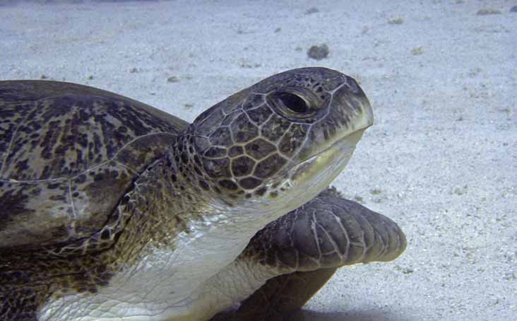
7
MARINE TURTLES
7.1 INTRODUCTION
Globally, there are seven species of sea turtle: the
leatherback Dermochelys coriacea (Family Dermochelydae),
loggerhead Caretta caretta, hawksbill Eretmochelys imbricata,
olive ridley Lepidochelys olivacea, Kemp's ridley Lepidochelys
kempi, green Chelonia mydas and the flatback, Natator
depressus (all in the Family Cheloniidae). The status of an eighth
species, the black turtle Chelonia agassizii is currently the
subject of debate among biologists, having first been described
by BOCOURT (1868) but later disputed by BOWEN et al. (1993).
The Convention on International Trade in Endangered Species
of Flora and Fauna (CITES) lists all marine turtles on
Appendix 1 (prohibited from international trade). The World
Conservation Union (IUCN) lists the green, loggerhead and
olive ridley as `Endangered', the leatherback, Kemp's ridley and
hawksbill are listed as `Critically Endangered', and the flatback
is listed as data deficient, whereby there is insufficient data to
determine its status.
Turtles have been used as a source of food and for other
commodities. Trade in turtle products has focused mainly on
their carapace, meat, oils and leather. Turtles also provide
revenue through tourism, and are important for research,
education and employment. Turtles are keystone species,
207

---

Standard Survey Methods
important for the health of the ecological
elsewhere (possibly feeding grounds off
system. Turtles have immeasurable value as
Oman or Pakistan). In turn, turtles foraging in
cultural assets and can act as flagship species
the RSGA region may migrate elsewhere to
in local and regional conservation projects. To
nest. This raises international conservation
conserve turtles and their habitats, extensive
issues that extend beyond the region.
marine areas must be taken under
management. This helps protect a range of
natural ecosystems and resources in this
Hawksbill turtles are circumtropically
complex and interconnected world.
distributed and have been studied in Oman
(ROSS 1981), Sudan (ABDEL LATIF 1980;
HIRTH & ABDEL LATIF 1980), Yemen (FAO
The Red Sea and Gulf of Aden (RSGA)
1973; GREEN 1996), Egypt (FRAZIER & SALAS
region supports five turtle species: the green,
1984) and Saudi Arabia (MILLER 1989;
hawksbill, loggerhead, olive ridley and
PILCHER 1999). Hawksbills inhabit coral reefs
leatherback (GASPARETTI et al. 1993). Only
where they feed primarily on sponges
the first three are known to nest within the
(MEYLAN 1988). These habitat assemblages
region. The status of marine turtles in the
are widely distributed throughout the region,
region was summarised by ROSS and BARWANI
making studies of hawksbills at feeding
(1982). This study is still considered one of
grounds difficult. In the RSGA region,
the most accurate regional reports available.
hawksbills tend to nest diffusely on isolated,
remote beaches. Hawksbills are believed to
make shorter migrations than other species,
Green turtle populations were first
and may thus remain closer to their natal
surveyed in detail in Saudi Arabia in 1986 and
beaches.
1987 (MILLER
1989). The National
Commission for Wildlife Conservation and
Development (NCWCD) carried out follow-
Loggerheads have been studied
up surveys from 1989 until 1997 (see AL-
extensively in Oman, where the world's
MERGHANI et al. 2000 for a review). Green
largest rookery is found (ROSS & BARWANI
turtles have also been studied in Yemen
1982). More recently, loggerheads have been
(HIRTH & CARR 1970; HIRTH et al. 1973), in
found to nest in Socotra and Yemen (PILCHER
the Egyptian Red Sea (FRAZIER & SALAS
& SAAD 2000). Records exist of migrations of
1984), Oman (ROSS 1984, 1985; SIDDEEK &
loggerheads from Oman to Socotra and parts
BALDWIN 1996) and Somalia (SCHLEYER &
of the eastern African continental coastline.
BALDWIN 1999). Green turtles are herbivorous
Loggerheads forage on a range of hard and
and spend the majority of their juvenile and
soft benthic habitats, primarily feeding on
adult lives foraging on shallow seagrass beds.
molluscs and crustaceans. As juveniles,
Due to the logistics involved with conducting
loggerheads typically forage in the open
fieldwork at these sites, studies at foraging
pelagic habitats of the Indian Ocean. Given
grounds are limited (HIRTH et al. 1973; ROSS
the limited mixing between the Red Sea and
& BARWANI 1982; AL-MERGHANI et al. 2000).
the Indian Ocean, it is unlikely that
Turtles are usually only accessible when the
individuals enter through the Bab el Mandeb
females emerge on beaches to nest. Green
except as strays. Loggerheads are not
turtles normally nest in large aggregations;
common in the Red Sea and probably do not
this makes nesting beach studies particularly
nest there.
useful. Given the long distance migrations
undertaken by green turtles, it is possible that
nesting females in the region originate from
208

---

Marine Turtles
Problem Survey
Method
Notes
Need to record and map
Desktop and literature
Provide information on previous studies in the
all areas of concern to
surveys
area on which to base further studies
turtle populations
Preliminary presence-
Identify where turtles are found
absence surveys
Rapid coastal surveys
Identify potential and actual nesting habitats and
their characteristics
Interviews
Provide subjective data on turtle distribution,
threats, species presence, etc.
Need to quantify nesting
Aerial surveys
Provide (limited) but high coverage information
on beaches
on nesting numbers and success
Detailed nesting beach
Provide accurate nesting volume and success
surveys
assessments, and options for reproductive biology
studies
Short term nesting beach Provide rough nesting assessments
inspections
Track counts (short- or
Provide relatively accurate nesting volume and
long-term)
success assessments and can be rapid
Need to quantify turtle
Aerial surveys
Provide counts of turtles at the surface for sampled
abundance at foraging
areas, which may be extrapolated to an estimate of
grounds
total abundance
Mark and recapture
Provide estimates of foraging population size
studies
through recaptures of marked individuals. Can be
resource and time consuming.
Need to identify
Tagging studies
Provide an option for recapture of individuals over
individual turtles
time
Need to discover
Tagging studies
Based only on recaptures and public participation
migration destinations
for tag returns (low cost)
Satellite tracking
Provide extremely accurate migration path
trajectories and destinations (expensive)
Need to determine short-
Radio or sonic tracking
Provides data on short distance movements of
distance movements
turtles, requires training and experience, can be
demanding on financial resources and time
Need to determine
Nesting beach surveys
Can evaluate nesting success, egg deposition,
reproductive success
incubation period and success, etc.
Need to identify diet of
Stomach content
Identification of stomach contents requires
turtles*
analysis
experience; must be performed by trained
personnel
Need to identify
Laparoscopy Surgical
procedure,
requires trained expert and
reproductive state of
laparoscope
turtles*
Need to identify impact
Observer programmes
Provide data on mortality and accidental captures;
of fisheries
can provide additional useful data
Need to determine
mtDNA and nDNA
Requires small samples, which can be collected by
genetic affiliation of
analysis
field researchers; analysis requires laboratory with
turtles
trained technicians
Need to identify sex
Histology studies Requires
sacrificing hatchlings for gonad
ratios of hatchlings*
inspection; requires training and experience
Table 7.1 Questions related to marine turtle populations in the RSGA region and suggested survey methods
to fill gaps in knowledge. Those marked with a * require significant training and should only be conducted with
the assistance of experienced professionals.
209

---

Standard Survey Methods
Olive ridleys are known to nest in Oman
7.2 DESKTOP SURVEYS
but at no locations in the RSGA region (ROSS
& BARWANI 1982). They are omnivores
In a desktop survey, literature should be
concentrating on molluscs and crustaceans. It
reviewed to obtain existing information on the
is possible that they forage in Gulf of Aden
region. This will help identify gaps in
waters where they may be subject to fishery-
knowledge and identify where to concentrate
related accidental mortality. Olive ridleys
future survey efforts. Information will be
share the same developmental habitats and
found in international journals and also as
geophysical constraints as loggerheads. They
internal reports. Access to a vast literature
are also not present in significant numbers in
base is now available through the internet.
the Red Sea.
The main resource is the Sea Turtle list-server
called CTURTLE, which one can join by
sending a message to <owner­cturtle
The leatherback has been documented in
@LISTS.UFL.EDU> or by following the
northern Red Sea and Gulf of Aden waters.
links on the web pages listed below:
However, is not known to nest in the RSGA
region. The leatherback feeds primarily on
www.seaturtle.org
jellyfish, which are abundant in the Gulf of
Aden waters during the monsoonal upwelling
www.turtles.org.
season. This is also a period of heavy fishing
pressure and the leatherback is threatened by
The Sea Turtle Online Bibliography,
entanglement in fishing gear. Leatherbacks
maintained by the Archie Carr Centre for Sea
are known to make long migrations and turtles
Turtle Research (ACCSTR) has thousands of
in the RSGA region may originate from the
up to date records. Internet access procedures
Andaman Islands in India or from South
have been improved through the WebLUIS1
Africa.
interface and there are now more advanced
search capabilities. The Sea Turtle Online
Bibliography web site contains access
Table 7.1 provides an overview of the key
information and links to further information
questions facing researchers and suitable
(web page: accstr.ufl.edu/biblio.html).
survey methods for providing answers. These
survey methods are based almost entirely on
those described in ECKERT et al. (1999) and
Maps and charts can often highlight
references therein. The following sections
potential nesting areas. For example,
provide detailed step-by-step methods for
mangrove-fringed coasts typically do not
carrying out surveys that will provide
support nesting, but island habitats often do.
adequate data to determine the status of
Extensive shallow areas along the coast
marine turtles in the RSGA region. Each
generally represent shallow muddy substrates
method is preceded by a brief introduction
unsuitable for nesting. It is important to
and, where applicable, a description of ways
ground-truth information taken from maps
in which the results can be used for
and charts as these are not always at a scale
management decision making.
that can reveal specific coastal types.
1 The WebLUIS interface is being phased out. Access may be made via the University of Florida Database Locator at
web.uflib.ufl.edu/locator.html. Search for the 'UF Sea Turtle Bibliography'.
210

---

Marine Turtles
7.3 INTERVIEWS
When was the last time you saw them?
Interviews should be used when little or
Do they nest in large numbers, or just
no formal reports exist for the area. Interviews
a few at a time?
should not be restricted to fishermen, because
Do you see more than ten in one night?
other coastal residents (such as coastguards
and ship crews) may have knowledge of
Where are the beaches where you see
turtles in their region. A series of questions
the turtles?
about turtles, such as species present,
seasonality, egg laying and threats should be
Could you show us the beaches where
posed to obtain basic, unbiased information.
you see them?
The interviewer should carry identification
Do people eat turtles? What about
sheets and photographs of different species in
their eggs?
and out of the water (see Appendix 7.12.1).
Are turtles used for anything else?
Interviews can take the form of formal
Have the numbers of turtles increased
questionnaires with a pre-prepared list of
over the years?
questions. However in the RSGA region,
Do you think there is anything that
simple discussions with the local residents
might be killing turtles and reducing
have proven more useful. It is important to
their numbers?
keep in mind the basic questions for which
answers are sought, but informal discussions
How would you feel about helping to
often reveal more accurate information. When
protect sea turtles?
asking questions it is important that the
interviewee feels relaxed and is not
intimidated, for instance when asking
7.4 PRELIMINARY SURVEYS
questions on exploitation. Questions that must
be incorporated into informal discussions are:
Long-term conservation of sea turtles
Do you see turtles nesting/swimming
depends on the availability of suitable nesting
around here?
beaches. Therefore, it is useful to determine
the location of nesting habitats and the size of
If so, where do you see them?
nesting populations. Records need to be
gathered on habitat area and type, ownership
Are they all the same kind, or do you
and conservation status, along with notes on
see different types of turtles?
anthropogenic and natural threats. The
What names do the turtles have?
existence of many kilometres of sandy beach
does not guarantee the existence or suitability
Do they look like any of the ones on
of nesting habitat. One must first identify
these graphics/photographs?
potential sites through literature searches and
interviews, and then carry out surveys by boat
Can you match your turtle names with
or airplane. Whichever method is used,
the pictures?
surveys must be cost-effective, reproducible,
Is there any particular time of the year
quantitatively rigorous and easily taught to
that you see turtles?
others.
211

---

Standard Survey Methods
7.4.1 Preliminary nesting beach surveys
Define the survey area.
on the ground
Partition into smaller sub-units, no
These are possibly the most widely used
longer than 1 km (use long-lasting
type of survey because turtles emerge onto
markers, or take bearings on permanent
land to nest and can then be easily studied.
structures, or use GPS).
Surveys over several seasons can give an
Carry out patrols shortly after sunrise,
indication of trends in the size of nesting
when tracks are still fresh (the sun dries
populations, which may be correlated loosely
the sand and tracks become obscured).
with overall population sizes. Ground surveys
are used when the beach is accessible and
If other beach survey efforts are
relatively short, or if there is a need to study
underway, track counts can be done at
the nests themselves (e.g. for nesting success).
night, although one runs the risk of
They are also used when air surveys are
disturbing nesting turtles.
unsuitable, for example due to obstructions, or
when crawls (tracks) cannot be identified
Move along the latest high tide line.
from the air (such as on rocky or pebble
Record the number and type of crawls,
beaches, as on Socotra). Surveys can occur
nesting pits, eggshells and slaughtered
over the long-term and be highly structured,
turtles.
or can be rapid `snapshots' of the current
situation.
Distinguish between fresh crawls
(those returning through the previous
night's tide line) and old crawls. This
Ground surveys cover the coastline
allows a count of the number of turtles
looking for signs of nesting. The most obvious
nesting the night before, and the total
signs to look for are the presence of tracks, but
over the last few days. Driving the
other information can also be collected. For
length of the beach the day before the
example, the species of turtle can often be
crawl count `marks' all existing tracks.
determined by the size and type of the tracks.
Only tracks that cross the vehicle
Hawksbills are small and walk with an
tracks will be `fresh' on a subsequent
alternating gait leaving narrow asymmetrical
count.
tracks; greens are large and walk with a
simultaneous gait, leaving wide, symmetrical
Identify direction sand is pushed and
tracks. Similarly, the success of the nesting
thus direction of crawl.
attempt can often be determined by looking at
Follow emerging crawl and look for
the nesting pit. Predominant threats should be
loose sand covering the crawl.
noted, as well as ownership of the site.
Normally patrols are carried out on foot.
Look for loose sand `plume' from
When the area is large, one can use four wheel
filling-in process (sometimes more
drive `All Terrain Vehicles' (ATVs) for
damp than surface sand) and for a
patrolling the beach. ATVs have large,
secondary body pit.
balloon-type tyres that prevent getting stuck
Determine if the emergence resulted in
in the sand. These specialist tyres do not
successful nesting. Also record the
damage eggs incubating in the sand if a nest is
number of unsuccessful pits (if any) the
accidentally driven over. The researcher
turtle excavated. False crawls tend to
should be equipped with predesigned data
have unfinished primary pits, often
sheets, pencils and camera. Survey
with a partially excavated egg
methodology is outlined below:
chamber. Note possible signs of
212

---

Marine Turtles
disturbance. Frequently the turtle
Beach slope
makes a number of unsuccessful body
pits before returning, or before finally
Beach composition (grain size,
nesting successfully. Note: it is
type, compaction)
important on high density nesting
Wave conditions and patterns
beaches to be careful when following
the tracks of turtles that have attempted
Presence/absence of rivers
to nest, moved a few metres, and
attempted to nest again, as tracks can
Presence/absence of man-made
easily get confused.
structures
Check the length of the crawl (if return
Potential threats
is a lot longer than emergence, it is
probable that the turtle spent a long
7.4.2 Preliminary beach patrols by
time on the beach and there is a good
aircraft
chance she nested. Caution: she might
only have been wandering or digging
Aerial surveys are typically used for large
unsuccessfully).
areas. Helicopters are the best option as they
If predators have excavated nests, they
can hover and fly at slow speeds. However,
should be marked as successful nests,
they are more expensive and not always
with an additional comment on
available. Single engine, wing above cockpit,
predation (as the turtle did indeed lay
aircraft are the most widely used for aerial
eggs).
surveys. Typical methodology is as follows:
When nesting success is not certain,
Determine survey area.
mark nesting success as unknown.
Keep speed in the range of 80­100
Mark each track after it is recorded by
knots (it is hard to count tracks at any
scraping a line through it with a stick.
higher speed).
This will avoid duplicate counts of the
same track.
Keep altitude between 50 and 300 m
(the greater the altitude, the larger the
Determine the species by track type.
field of view, but the less discernible
Use results from the counts to
lighter tracks are, such as hawksbill or
determine the number and density of
olive ridley; optimal altitude should be
turtles nesting in each area. Over the
around 150 m).
course of several seasons, these data
Aircraft must maintain constant speed,
can also provide an understanding of
height and relative position to the
inter-seasonal fluctuations.
shore while maintaining safety.
Record the following beach
Position the aircraft so that the
characteristics:
observer can see the beach clearly.
Location (GPS)
Usually this can be done by keeping
the craft 0­20 m offshore, where the
Vegetation type
observer can see tracks emerging and
returning to determine nesting success.
Beach length
Keep all surveys less than two to three
Beach width
hours in duration to avoid fatigue.
213

---

Standard Survey Methods
Have two or more observers who do
Nesting density. High-density beaches
not communicate their results during
are not good for aerial surveys, as the
the flight to test for observer
observers tend to get confused
differences / errors / biases. Observers
counting tracks that overlap.
should be well trained and highly
experienced in identifying the
Beach type. Grain coarseness can
characteristics and types of nesting
affect the impressions made by turtles
crawls and nesting marks.
during the crawl.
Carry out surveys at dawn, when
Time of day. The angle of the sun
shadows on the tracks are most visible.
might make it hard to see tracks if
there are no shadows.
Schedule flights on the mornings
before, on, and after the day when
Weather. Wind and rainfall might
spring tides peak after about 1900 to
erode tracks away.
2000 hours (this way the tide will be
Human activities. These may obscure
'in' during the night, and then 'out' for
tracks and pits.
most of the early morning and during
the surveys, and data can be averaged
for the three-day results).
Therefore, aerial surveys in particular
require ground-truthing. This involves
Search for tracks that extend below the
comparing data collected by aerial observers
latest high tide line.
or other beach monitoring efforts with data
collected by an experienced researcher on the
Determine nesting success and
ground. This can be established through the
species.
presence/absence of eggs on studied beaches.
Mark nests as successful, unsuccessful
or unknown.
Identify beaches where nesting was
thought to have occurred.
7.4.3 Ground-truthing
Locate what are thought to be
successful nests.
The accuracy of counts from aircraft, or
those conducted by trainee researchers, must
Dig gently by hand a small hole in the
be ascertained in order to achieve acceptable
area that is thought to contain eggs.
results. Factors affecting accuracy include:
When reaching nearly one arm's
length, continue slowly and carefully.
Observer accuracy. For instance, each
observer may record different numbers
When eggs are encountered
of crawls, or misidentify the species.
immediately re-cover the nest and
mark it.
Turtle species. Hawksbills are lighter,
and leave a much `shallower' track,
Identify differences between ground-
also they tend to nest close to
truth data and aerial survey / trainee
vegetation and pits might not be
field data. Errors between both data
visible.
sets then yield an error factor, which
must be considered in all subsequent
estimates.
214

---

Marine Turtles
7.4.4 Preliminary foraging area surveys
have shorter flight ranges. Whichever is used,
flight attitude and altitude should be
Sea turtles spend most of their lives in the
maintained constant to allow standardisation
water, such as in coral reef and seagrass
of observations.
habitats. The number of studies that can be
carried out in these habitats is significantly
reduced because of the logistics involved,
7.5.1 Aerial surveys of nesting beaches
costs, etc. Potential foraging areas should be
visited using snorkel or scuba equipment.
When surveying nesting beaches, it is
Survey methodology is outlined below:
useful to have maps or charts for the area to be
surveyed prepared in advance. Photocopy
Record the presence of foraging turtles.
maps into manageable A4 or A3 size and stack
these in sequential order. As the aircraft flies
Record area location (GPS), relevant
along the coast, keep track at all times of the
underwater life forms (seagrasses,
location by referring to major landmarks on
sponges) and physical characteristics
the charts, flipping to the next chart as land
(currents, depth, water temperature,
area is covered.
benthic structure).
Turtle densities should be established
using line transects and quadrat
7.5.2 Aerial surveys of foraging grounds
methodology (see chapters on Rapid
These methods work because turtles
Assessment and Corals and Coral
surface to breathe, at which point they can be
Communities).
counted during strictly timed `passes' or
Capture turtles using nets or rodeo-style
transects. Turtles are counted and where
captures (see below).
possible, species identified. The number of
sightings in a set area (the sample) can then be
Use mark and recapture studies (see
extrapolated to cover wider areas to arrive at
below) to provide information on
an overall area estimate (the population). Due
abundance, distribution, size classes
to the difficulties in observing turtles and
and species.
identifying species, surveys must use trained
observers. The aircraft (single engine for
nearshore, twin engine for offshore) should
7.5 AERIAL SURVEYS
have easy line-of-sight to the sea surface,
through Plexiglas windows in the nose or
floor or protruding bubbles. Planes should be
Aerial surveys are generally expensive,
equipped with a GPS navigation system.
but provide extremely wide area coverage in a
Transect (flight line) length should be
very short time. Often, when the costs of
determined after taking into consideration the
mounting large-scale ground projects are
area to be surveyed, time available, and
compared with two or three days of aerial
overall objectives. The best results are
surveys, the latter is found to be the most cost
obtained when more than 30 turtles are
effective. Surveys can be done from a small
identified. In conjunction with field studies,
airplane or by helicopter, the latter having the
which determine the average proportion of
option of landing at selected sites for closer
time spent at the surface for the species in
inspection. Airplane surveys are fast and can
question, the results of these surveys can be
cover a large area without landing.
extrapolated to include turtles that may have
Helicopters need to refuel more often and thus
been submerged during flight overpasses.
215

---

Standard Survey Methods
Aircraft preparation
Mark the window with a greaseproof
Mark aircraft windows to provide a field of
pencil where the reference line is again
view in order to survey the area quantitatively.
seen, to identify the outer boundary of
This will establish a sector through which the
the survey zone.
viewer should focus attention. The sector
should be of a known width.
Repeat for the other side of the aircraft.
Carry out a test flight at the
predetermined altitude (e.g. 150 m) in
a straight line as close as possible to a
The total area covered by each flight
known long reference line (such as a
transect (A) can then be calculated using:
straight road), so that the observer can
see the reference line straight below
A = wL
the aircraft (Figure 7.1a).
where:
Mark the window with a greaseproof
pencil where the reference line is seen,
w = the width of the viewing area
to identify the inner boundary of the
(equal to the perpendicular
survey zone.
distance away from the reference
line) and
Have the pilot move perpendicularly
away to the limit of the observer's field
L = the length of the individual
of view through the window and
transect.
determine the straight-line distance
from the reference line (using the
aircraft's GPS) (Figure 7.1b).
a
Reference
line
path
Flight
path
Mark inner field
of view line
b
Reference
line
Flight
path
Mark outer field
of view line
Figure 7.1 Aircraft setup:
a ­ fly along reference line and mark proximal survey area limit on
window;
b ­ move horizontally away to distant limit of the field of view and mark
outer limit of survey area.
216

---

Marine Turtles
Survey flight methods
7.5.3 Additional data collection
Transects should be parallel to each
other, and perpendicular to the depth
During aerial surveys of open water
contours.
habitats, data on other marine animals can be
collected, given the low density at which these
Flights should be planned with safety
and turtles are encountered. Therefore, aerial
in mind and carried out in calm
surveys can be used to determine the
weather (Beaufort Sea State 2), as
distribution and abundance of turtles, whales,
turtles are difficult or impossible to
dolphins and dugongs all in the same project
spot in rough sea conditions.
(see chapter on Marine Mammals).
Flights should be conducted close to
noon (12:00 hours) to minimise glare.
7.6 NESTING SEASON
Have one observer on each side of the
aircraft.
SURVEYS
Where possible, have one additional
Estimating population numbers is useful
observer in a front seat taking
in conservation programmes to help
independent recordings, to check
understand long-term trends in population
against the rear observer.
size and the severity of threats (small
Observers should attempt to identify
populations are in more danger than larger
the species based on silhouette (see
ones). One can count absolute numbers (e.g.
Appendix 7.12.1), or at least identify
total number of females) or relative numbers
between hard shelled and leatherback.
(e.g. number of nesting females or number of
nests). One can also count emergence tracks
Keep all surveys to less than 2­3 hours
to determine relative nesting population sizes.
to avoid fatigue.
In all cases one must consider bias (measured
as closeness to actual figure) and precision
Record number and species (where
(measured by the variance). For example,
possible) of turtles in each transect.
aerial surveys are imprecise and biased
From transect surveys, compute a
(turtles are rare and the results are always
population estimate (C) using:
underestimated), while comprehensive nest
counts are precise and unbiased (one can
C = (n / 2 wlg) A
count each nest and the results among
different researchers would nearly always be
where:
the same).
n = number of turtles counted
l = length of transects
An understanding of reproduction and
nest biology is a valuable tool for
w = width of transects
conservation and management of sea turtle
g = fraction of turtle population
stocks. Without this knowledge, well
visible
intentioned, but ignorant, conservation efforts
can be detrimental to sea turtles. The nesting
A = size of study area (from
beach provides a narrow but important
above).
window for studying sea turtles.
217

---

Standard Survey Methods
When studying nesting populations, one
flashlights, preferably with a red filter, and
needs to bear in mind that the number of
movements by personnel in the vicinity of
nesting turtles varies annually, often to
turtles should be slow and deliberate, as
extremes. For example, at Ras Baridi on the
turtles are sensitive to light and movement.
Saudi Arabian Red Sea coast, nesting
numbers have fluctuated from 110 individuals
one year to only 17 the next, and back up to 73
Long-term comprehensive nesting surveys
the following year. This is a normal
These surveys target nesting beaches with
occurrence and is used to highlight the need
significant breeding populations, or beaches
for long-term studies (decades) at nesting
that host the only known nesting population.
beaches to determine any trend in population
They are time and labour intensive and
size. If one were to record the numbers of
require a significant degree of planning and
turtles during a `bad' year, this would give a
logistical arrangement. At night researchers
false underestimate of the average nesting
should monitor all or parts of the nesting site
numbers, while similar work during a `good'
and collect data on nesting numbers, turtle
year might yield a false overestimate. In
morphometrics (size measurements, weight),
addition, marine turtles do not nest every year
damage to turtles, number of eggs laid, nest
(typically there is a three to five year interval).
location and a number of other variables.
Thus, understanding annual variation in
During the day data can be collected on turtles
numbers of nesting females requires
not sighted during the night surveys, beach
comprehensive beach coverage for most of
area and morphology, sand characteristics,
the nesting season and monitoring surveys
males (by rodeo capture), and inter-nesting
that extend over several years. While one-
habitats (see methods below).
season nesting surveys cannot provide reliable
data on population size, they can give useful
information on female nesting biology and
Peak nesting season surveys
overall reproductive output, as well as threats
To minimise survey effort, it is often
and conservation needs. Additionally, they
possible to concentrate studies on turtles
provide a useful platform on which to base
during the three to four weeks at the peak of
public awareness and beach conservation
the nesting season. This can only be done
projects.
when a substantial amount is known about the
nesting populations, as in Saudi Arabia. For
instance, knowing that green turtles nest on
7.6.1 Survey timing and duration
Karan (Arabian Gulf) from May to
September, with a peak in July, allows
Surveys should be timed so that they start
researchers to target this month rather than
at or near the beginning of the nesting season.
spend four months on the island. During this
This can be determined from earlier
time up to 80% or 90% of the nesting
interviews, nesting at nearby sites or through
population can be encountered.
previous reports. Turtles are generally
nocturnal, although they do occasionally nest
during the day. Beach surveys should be
7.6.2 Location information
carried out at night, starting from shortly after
sunset until no further turtles are encountered
Standardise the nesting location name.
on the beach. Periodic but less frequent
Location can be further subdivided
surveys should also be carried out during the
into sites (for instance, an entire island
day to detect daytime nesting activity. Lights
may constitute a location, while the
should be restricted to small penlights or
North, East, West and South might
constitute sites).
218

---

Marine Turtles
Identify individual beaches, and
The tag can be recovered easily when the
subdivide beaches by sectors (where
nest is excavated, by searching for the
the beaches are longer than 1 km).
coloured tape. Where egg poaching is
common, nest locations must be recorded
without allowing for detection. This can be
7.6.3 Nest characteristics
done by measuring distances and angles
Record the exact nest location (useful
(transits) to at least two nearby immobile
for returning to the same nest at the
objects such as large rocks, trees or headlands.
end of the incubation period to
determine incubation success). The
Draw a diagram showing the
particulars of each nest allow a
approximate location of the nest.
comparison among populations and
can provide a descriptive summary of
Measure carefully and record the
the physical characteristics of nests.
distance from the nest to one of the
reference points using a long tape
Measure nest depth from the top of the
measure. Measurements must be
sand (average beach surface) to the
accurate as the beach may change
bottom of the egg chamber and also to
shape through erosion and other
the top of the uppermost egg. Take
nesting activity over the next 60 days.
measurements using a flexible
fibreglass tape measure (±1 mm) as
Repeat for the second and subsequent
the turtle completes the chambering
reference points.
process and then again after the last
egg is deposited, but before filling-in
When relocating the nest, attach the
commences.
tape measure to the first reference
point, then extend it to the distance
Attach an identification marker to a
recorded earlier in the general
1 m piece of coloured tape.
direction of the nest and mark an arc in
the sand.
Insert the tape and tag plate as the
turtle deposits the eggs.
Repeat the procedure for the second
and subsequent measurements from
Record an individual nest identification
reference points.
number on the marker, in permanent
ink.
Relocate the nest by finding the point
at which the measured transits cross
Maintain a database of nest data, to
(Figure 7.2).
include the following information: tag
number; date and time laid; nest depth
(top and bottom); nest location
7.6.4 Nesting turtles
(according to sector code or
triangulation coordinates ­ see below);
Generally only female turtles emerge onto
nest habitat type (open beach,
nesting beaches, although sometimes males
vegetated beach, etc.); sand
emerge while still in a copulating position
temperature; clutch count; egg
mounted on the female. Consequently much
diameter and egg weight.
more information has been collected for
female turtles than for males. Adults are
Cross-reference the nest number to the
measured to provide an indication of general
tagging data for the female that
population characteristics, to determine the
deposited the eggs.
minimum size at maturity and for subsequent
219

---

Standard Survey Methods
re-measurement at later dates to enable
carapace with a fibreglass tape measure (±
calculations of growth rates. They are usually
0.1 mm). Straight length measurements are
tagged to provide individual recognition in
taken with callipers (± 0.1 mm) to record the
subsequent recaptures and to prevent re-
straight-line distance between one point and
sampling of the same individual. Female
another. The arms of the callipers should only
turtles can be identified using the diagrams in
be as long as necessary, to reduce bulk and to
Appendix 7.12.1.
increase accuracy. The length should only be
slightly larger than the maximum expected
size and all records should be able to be taken
7.6.5 Morphological data
in a single attempt, rather than several partial
measurements. Any barnacles or other
Turtles are measured on nesting beaches
organisms growing where measurements are
to relate body size to reproductive output, at
to be taken should be removed with pliers
foraging grounds to determine frequency of
beforehand. A sample data sheet for recording
size classes (to determine demographic
nesting data is presented in Appendix 7.12.2.
structure), and to monitor growth rates (in
The following are the most common
subsequent recaptures). It is important to
measurements recorded for sea turtles.
ensure accurate measurements are taken and
recorded. Practice measurements can be made
Curved Carapace Length (CCL) ­
on a turtle carcass or a sample turtle. The
measured over the curve of the
sample size should also always be reported so
carapace along the midline from the
that one can determine the validity of the
anterior point at the midline of the
summary data. An average taken among four
nuchal scute to the posterior tip of the
individuals will not be as precise as an
surpacaudal scutes (Figure 7.3).
average taken from 100 individuals. It is best
to have one researcher take all measurements
Curved Carapace Width (CCW) ­
all the time to ensure consistency in
measured over the curve of the
methodology. If this is not practical, different
carapace perpendicular to the midline
researchers should practice and standardise
across the widest portion of the
methods prior to actual data collection.
carapace (Figure 7.4).
Consistency in measurement taking is critical
for later comparisons and analysis. Curved
Straight Carapace Length (SCL) ­
measurements are taken over the curve of the
measured as a straight-line distance
Inland rocks
Inland rocks
Nesting beach
The nest is located at the point where
the two measured transit lines cross.
Transit points
Figure 7.2 Nest relocation technique using permanent transit points
220

---

Marine Turtles
For leatherbacks, curved measurements
Straight carapace length
are not taken on the top of the carapace ridges
due to shape irregularities. The curved
Curved carapace
measurement is taken as in the case of hard-
length
shelled turtles, but the tape is allowed to run
along one side of the dorsal ridge. Curved
width is recorded from side to side over the
tops of the ridges, at the widest point. Straight
Figure 7.3 Curved and straight carapace length
length is measured from the anterior edge of
measurements
the carapace at the midline to the furthest
point on the caudal peduncle. Plastron
between the anterior point at the
measurements are not practical and are
midline of the nuchal scute to the
therefore not taken.
posterior tip of the surpacaudal scute
(Figure 7.3).
7.6.6 Weight
Straight Carapace Width (SCW) ­
measured as a straight-line distance
Turtles should be weighed with a
between the outer edges of the
saltwater-resistant spring balance (±0.5 kg).
marginal scutes at the widest portion
The easiest way to weigh turtles is to form a
of the carapace perpendicular to the
figure of eight with a sturdy piece of rope
midline (Figure 7.4).
measuring about 2 m in length. One end of
Plastron Length (PL) ­ measured
the loop should be slightly larger than the
along the midline from the joining of
other and the cross point should be tied tight.
the skin and plastron at the anterior
After carefully flipping a turtle onto its back,
edge to the posterior-most projection
the smaller loop can be placed over the front
of the bone. If the turtle is not turned
flippers and head to support the anterior
over for weighing, this length need not
portion of the carapace. The larger loop is
be taken (Figure 7.5).
looped over the rear flippers and tail and
supports the posterior of the carapace. A
Plastron Width (PW) ­ measured
balance is positioned at the cross point and
across the plastron at its widest point
supported with a sturdy brace, which is then
perpendicular to the length. If the
lifted by two people (Figure 7.7).
turtle is not turned over for weighing,
this measure need not be taken
(Figure 7.5).
Head Width (HW) ­ a straight distance
Straight carapace width
across the widest portion of the skull.
Curved carapace
Care should be taken when taking this
width
measurement as the turtle's ears are
hidden behind the large lateral scales
posterior to the eyes.
Tail Length (TL) ­ measured from the
tip of the tail to the trailing edge of the
Figure 7.4 Curved and straight carapace width
plastron (Figure 7.6a) and from the tip
measurements
of the tail to the cloaca (Figure 7.6b).
221

---

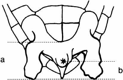
Standard Survey Methods
maximum), standard deviation (SD)
and sample size (n) (using a suitable
spreadsheet programme).
Plastron
Present morphometric data in tabular
length
form (see example presented in Table
7.2 below).
Use morphometric date to describe the
basic parameters of the population.
Long-term data sets can be used to
Plastron width
monitor recapture rates of previously tagged
turtles, which can be indicative of tag-loss
rate. An example of the manner in which this
Figure 7.5 Plastron length and width
is presented is shown in Table 7.3. A
measurements
consistently low recapture rate may suggest
overfishing and exploitation if recaptures are
During initial surveys it is suggested that
constantly low (such as the example in
as many turtles as possible be weighed. Not
Table 7.3).
all turtles need to be weighed during
subsequent surveys; a sample of 10­20% of
the population will provide a suitable
estimate.
Lift here
Lift here
Morphometric data are used to compare
populations from different years and different
locations, both regionally and globally.
Figure 7.7 Weighing a turtle
Summarise data from each nest for
each site.
Present morphometric and weight data
7.6.7 Tagging
as averages (x) for the whole sample,
noting the range (minimum and
Tagging turtles is a useful research tool
but is not a necessity for nesting beach
studies. If the objective is simply to count
turtles, short-term recognition can be
achieved using spray paint to mark the
carapace. This typically lasts about two weeks
in the natural environment. For a tagging
programme to be effective there must be a
commitment to future surveys and tag returns.
Tags, if used, should conform to the following
characteristics:
Figure 7.6 Tail measurements
222

---

Marine Turtles
Tags should be made of titanium (this
Mark one side of the applicator with
metal has shown some of the greatest
paint to identify the top position.
resistance to corrosion, and is among the
longest lasting underwater) and can be
Tape tags together on their cardboard
purchased from Stockbrands Pty (Fax
sleeves to reduce tag loss and maintain
69­9­444­0619).
tag order.
Numbers should be consecutive and
Check turtles for presence of previous
prefixed by the country's international
tags or signs of tag loss prior to placing
ISO code.
new tags, and keep notes.
Researchers are responsible for ensuring
Replace old tags only if they appear
that tag numbers are not duplicated
heavily corroded and might be lost easily.
within a project or among projects.
Record all previous tags to maintain a
Half the tags should bear the message
long-term history of the turtle.
"Notify PERSGA PO Box 53662 Jeddah
Turtles that show signs of having been
21583 KSA" in English, the other half
tagged previously but which have lost
should bear the same message in Arabic.
their tags should also be recorded as
Apply one of each to each turtle.
such, as this provides information on the
Do not order double sets of tags (i.e.
rate of tag loss.
bearing the same number), or attempt to
Tag new turtles on the proximal trailing
tag a turtle with the same number on each
edge of each front flipper (Figure 7.8) to
flipper (this is unnecessary and increases
reduce the chances of abrasion,
the risk of two turtles accidentally being
entanglement and tag dislocation.
tagged with the same number).
Tagging is a two-step process:
clamp applicator so that the sharp
Tagging should follow the methods outlined
point pierces the flipper and
below:
apply greater force to ensure the tag
Practice with several tags on a piece of
point bends over and securely locks
cardboard prior to working with turtles.
into rear of tag.

CCL CCW
SCL
SCW
PL
PW
HW
TL
WGT
X
94.30 85.80 86.30 69.10 75.00
65.50 17.50
15.70 94.50
SD
4.26
3.27 5.16
2.53
9.09
10.09
1.64
2.71
6.52
Max
103.00 93.00 91.00 73.50 91.50
89.00 21.00
21.00 108.00
Min
79.00 79.00 70.00 64.00 62.00
6.00 12.50
10.50 84.00
N
49.00 49.00 15.00 15.00 49.00
49.00 49.00
49.00 11.00

Table 7.2 Morphometric summary of adult loggerhead turtles in Socotra. x = Average; SD = Standard
Deviation: n = Sample size; CCL = Curved Carapace Length; CCW = Curved Carapace Width; SCL = Straight
Carapace Length; SCW = Straight Carapace Width; PL = Plastron Length; PW = Plastron Width; TL = Tail
Length; HW = Head Width (all in cm); WGT = Weight (kg).
223

---

Standard Survey Methods

Arabian Gulf
Ras Baridi

Chelonia mydas
Eretmochelys imbricata
Chelonia mydas
Season
New Recap Total New Recap Total New Recap Total
1986
1124 --
1124 15 -- 15 -- -- --
1987 330 0
330 20 0 20 15 -- 15
1988 -- -- -- -- -- -- -- -- --
1989 -- -- -- -- -- -- 61 0 61
1990 -- -- -- -- -- -- 16 1 17
1991 894
0 894 145
0 145 95 11 106
1992 512 18 530 123
4 127 19 15 34
1993 999 29
1028 34 3 37 27 8 35
1994 378 60
438 39 16 55 20 14 34
1995 346 85
431 34 21 55 13 7 20
1996 -- -- -- 31 17 48 -- -- --
1997 201 56
257 32 20 52 -- -- --
Total
4784 248
5032 473 81 554 266 56 322

Table 7.3 Suggested layout of tagging records over time.
Check carefully to ensure the tag is
Tag number and placement (i.e. which
securely attached, and that the sharp
flipper) should only be recorded after
point of the tag has looped through the
tagging has been completed
receiving hole and curved into a
successfully. Tags can break on
locking position (it is possible that the
application and must be discarded, and
sharp point curves back under the
it is possible to forget to change the
receiving side of the tag, or outside of
number if it is pre-recorded. Only the
it).
tag that is actually placed on the turtle
should be recorded.
Leave a 0.5­1.0 cm gap between the
trailing edge of the flipper and the rear
Copies of the tagging records should
edge of the tag when tags are applied
be submitted to PERSGA by the
to adult turtles (Figure 7.8).
researcher at the conclusion of each
research period, to maintain an up-to-
Leave a 1.0 cm gap between the
date database of tagged turtles in the
trailing edge of the flipper and the rear
RSGA region.
edge of the tag when tags are applied
to juveniles.
Only tag turtles when they have
completed covering the nest cavity
with the rear flippers to minimise the
Front Flipper
possibility of disturbing the turtle,
causing her to abandon the nesting
effort.
Turtle
Carapace
Tag turtles that emerge but fail to nest
when they are returning to the sea, as
they will usually return to nest at a
0.5 - 1.0cm
later time or date.
Figure 7.8 Tag position and gap between outer
edge of the tag and the trailing edge of the flipper
224

---

Marine Turtles
7.6.8 Determining clutch size
7.6.9 Measuring and weighing eggs
Clutch size is typically determined at
Eggs should be handled with caution and only
oviposition but if the nest has to be moved,
when necessary. Once a sample has been obtained,
eggs can be counted at that time. Clutch size
measured and weighed, quickly return the eggs to
should be determined for a minimum of 10%
the nest before completion of oviposition. Handle all
of the nesting population. It is useful to have a
eggs carefully with clean hands, without rotation and
mechanical counter, which is pressed each
only within two hours of when they were laid. Any
time eggs are deposited, because it is easy to
movement of eggs from this time for the next 25
miscount the number, and practically
days results in movement-induced mortality of the
impossible to recount without excavating the
embryos. Therefore, if the clutch will be affected by
nest after the female returns to the sea. The
tides and needs to be moved, this should be done
clutch size is defined as the number of normal
within two hours. The clutch should be moved to a
eggs and extra large eggs (as these may
location with suitable `nesting beach'characteristics,
contain multiple embryos) laid into the nest.
with regard to temperature, shade, moisture, etc.
Any turtle that lays a second clutch within six
days of the first was disturbed in the earlier
Clear a flat space close to the chamber and
attempt, and the two partial clutches should be
line with a plastic bag.
added together to obtain the actual clutch size
for that instance, provided the turtle was
Collect ten eggs at random as the female
marked and can be identified.
deposits the eggs into the nest chamber, by
digging a narrow tunnel through which the
Observe the female and wait until the
arm can be extended, and place them on the
chambering process is nearly
plastic bag.
complete.
Clean the eggs of any adhering sand.
Slowly crawl up behind the female,
Press gently on the egg so that the shell is
and wait until egg deposition begins
stretched tight, then measure and record the
(determining this takes an experienced
maximum and minimum diameters (across
researcher, but generally occurs when
axis at 90º to each other) using callipers
the female ceases the chambering
accurate to 1.0 mm or greater.
actions of the rear flippers, and draws
the rear flippers inward in a protective
Add the two values together and compute
manner over the nest cavity).
the average for each egg.
Shine a small flashlight directly into
Measure and record the weight of the egg
the nest cavity at close quarters,
on a spring or electronic balance accurate to
careful to avoid disturbing the nesting
0.5 g or greater.
female.
Repeat this procedure for all ten eggs.
Count the number of normal eggs
(normal shape and size, white,
Record data on a form such as that provided
spherical, and which have a yellowish
in Appendix 7.12.3.
hue when a flashlight is shone
Compute the mean and the standard
through) and odd-shaped eggs (these
deviation for the diameter and weight in
are small or extra large, or of different
each nest.
shape when compared with normal
eggs, and have a white hue when a
Use the nest averages to compute location
flashlight is shone through).
or year-class averages.
225

---

Standard Survey Methods
7.6.10 Measuring incubation
7.6.12 Measuring and weighing
temperature
hatchlings
Temperature of the sand affects embryonic
Hatchlings should be handled with caution
survival, hatchling sex and the duration of
and only when necessary. Natural dispersal of
incubation. The temperature usually varies
hatchlings from a nest site to offshore pelagic
within the incubation period and between
habitats involves a progression of behavioural
seasons.
responses, which are sensitive to disruption.
Hatchlings should not be detained following
Where equipment is available,
their emergence without a specific purpose.
incubation temperature should be
recorded throughout the entire
Measure ten hatchlings from at least
incubation period.
10% of all nests, as soon as possible
after emergence. Do not measure
Calibrate the thermometers prior to
deformed or `bent' hatchlings.
use at 15º, 20º, 25º, 30º, 35º and 40ºC
to establish any error in the devices.
Measure straight carapace length
(SCL) from the nuchal scute to the
Place the thermometers at a depth of
notch between the post-central scales
50 cm in the general area where nests
(as in measurements for adults, but
are deposited.
using small hand-held callipers
If nesting density is high, a sturdy
accurate to 1.0 mm or greater).
wooden stake should be driven into the
Measure straight carapace width
sand to a depth exceeding 1m and the
(SCW) at the widest point of the
thermometer or probe placed adjacent
carapace.
to the post, to prevent disturbance by
other nesting females.
Weigh each hatchling (out of the wind)
using a spring or electronic balance
Record temperatures daily at 0600,
accurate to 0.5 g or greater (care must
1200, 1800 and 2400 hours.
be taken to remove any adhered sand
before weighing). This job may be
simplified by placing the hatchling in a
7.6.11 Hatching and incubation success
container on a pre-tared1 balance, to
prevent the hatchling from crawling
The easiest method to determine nest
away.
incubation success is to compare the total
number of hatchlings that emerge from the nest
Record all measurements and weights
with the original number of eggs deposited.
for each hatchling on a data sheet such
Unfortunately, nests are often encountered
as that provided in Appendix 7.12.4.
hatching for which no original data are
available. It is rarely possible to collect all
Compute average and standard
hatchlings that emerge from a nest (unless they
deviations for each measurement for
are penned in), as they crawl rapidly to the sea,
individual nests.
and there may be multiple emergences from
Use nest averages to compute a
one nest over several days. It may therefore
location or year-class average.
prove necessary to excavate the nests.
1 Pre-tared: balance set to zero after container installed, or mass of container subtracted from gross weight of hatchling +
container.
226

---

Marine Turtles
7.6.13 Determining hatching and
To assess incubation success, one must
emergence success
establish hatching success (the number of
hatchlings that emerge from the shells) and
After incubation and hatchling emergence,
emergence success (the number of hatchlings
nests should be excavated to determine the
that reach the beach surface). Hatching and
following:
emergence success can be computed using:
(E)
number of hatchlings actually
leaving the nest
Hatchling success (%) = (S / (S + UD +
UH + UHT + P)) × 100
(S)
number of empty shells - only
count those that are more than
50% complete, do not count
Emergence success (%) = (S ­ (L + D) /
small fragments
(S + UD + UH + UHT + P)) × 100
(L)
live hatchlings left in the nest
(D)
dead hatchlings in the nest
7.6.14 Determining reproductive output
(UD)
the unhatched eggs with no
The reproductive output of a population
obvious embryo
may be used to make inferences on the quality
of the nutrition available to turtles. As turtles
(UH)
the unhatched eggs with obvious
nest many times in a season, the longer the
embryo (excluding UHT below)
duration of the survey the more accurate the
(UHT)
the apparently full term
data that can be gathered on the occurrence of
unhatched or pipped eggs
re-nesting. Determining clutch size and
hatching success provides invaluable
(P)
any eggs that have been
information related to the reproductive output
predated on (open, nearly
of nesting turtles, which is fundamental to
complete shells with egg residue
their conservation and management. When
inside).
reproductive biology data are analysed over
the long-term, they can provide the
foundation upon which management
Where the original number of eggs was
decisions are made. For instance, if the
known, this should be compared to the value
number of eggs deposited and which incubate
(S) to identify errors in nest excavation
successfully remains fairly constant, but the
counts. Where the original number of eggs
number of emerging hatchlings drops
was not known but all hatchlings were
dramatically, this indicates some sort of
counted, the clutch size (C) can be computed
problem with the nesting beach conditions
using:
(for example, cement dust at the Ras Baridi
site in Saudi Arabia). Similarly, reductions in
C = E + L + D + UD + UH + UHT + P
the number of hatchlings that reach the sea
could indicate an increase in natural
An estimate (N) of total clutch size (C)
predators, which would need culling or
can be computed if some of the hatchlings
controlling. Total reproductive output (O) can
were not found using:
be computed using:
N = (S ­ (L + D))
O = T × R × C × I
227

---

Standard Survey Methods
where: T = estimated number of turtles
(known as Ecologically Significant Units),
which can be identified on nesting beaches
and in foraging grounds. To identify discrete
R = average re-nesting occurrence
breeding populations, one needs to identify
the characteristics of the mitochondrial DNA
(mtDNA) molecule, which is a female-
C = average clutch size
inherited marker, and nuclear DNA (nDNA),
from which male-inherited information may
be determined. These two studies should be
I = average incubation success
conducted in a reputable laboratory by
qualified technicians. Genetic identification
of foraging populations is a priority activity.
Trends in reproductive output can be used
Samples can be taken from dried tissue on
to make assumptions indirectly on the state of
carcasses, small cuttings of rear flippers and
the environment. Coupled with data on
dead hatchlings or embryos. These can be
nesting turtles, long-term collection of data
stored dry and dispatched for analysis to
can suggest trends in population size,
major sea turtle research centres such as the
recruitment and mortality.
University of Queensland in Australia. All sea
turtles are listed under CITES and an export
and import permit will be required for
7.6.15 Re-nesting occurrence and
shipping samples for genetic analysis. Note:
interval
Each turtle must only be sampled once
Calculating the re-nesting interval (how
(on foraging grounds either mark with
many days between successive nests) can
paint or tag the turtles; for nesting
provide an indication of the impact of
turtles either mark the turtle or collect
research activities on turtles and on general
all samples within ten days to avoid re-
population condition. Typically turtles nest on
nesting occurrences by the same
a two-week cycle though in some parts of the
female).
world they nest on a four to five week cycle.
The re-nesting interval is calculated from the
Identify collection site and record GPS
time of the last successful complete nest to the
position.
first subsequent nesting attempt, regardless of
whether it is successful. This is because the
Use a large pair of nail clippers or a
simple act of emerging on the beach is already
sharp scalpel to remove approximately
an indication of the intent to nest. The interval
0.5 cm2 of tissue from one of the rear
is calculated in days and averaged for the
flippers.
population.
Store in a securely closing sampling
tube containing 70­90% ethanol or
isopropyl alcohol (pharmaceutical
7.7 GENETIC STUDIES
grade).
Clearly label the tube with a unique
Genetic studies have helped answer
number that identifies the donor turtle.
important questions with regard to turtle
Samples may then be correlated with
conservation. They have proven that female
location, gender, species, size class,
turtles return to their natal beaches to nest and
etc., at a later date.
that there are discrete nesting populations
228

---

Marine Turtles
Use new scalpel blades or clippers for
to shore. This method is only practical when
each individual to avoid cross-
there are no coral and rock outcrops to snag
contamination of DNA material.
the net when it is being retrieved. Given sea
turtles' ability and agility underwater, nets
should be relatively long (200 m or more),
7.8 FORAGING AREA SURVEYS
thus requiring several people for setting and
retrieval.
Foraging area surveys are used to study
turtles in their feeding areas underwater. They
are usually carried out by trapping turtles in
Foraging waters are often slightly deeper
tangle nets, in relatively protected, open,
than shallow, fringing lagoon waters and thus
shallow water areas, with little or no water
different types of nets are needed. Small purse
movement (currents). Turtles are tagged and
seines and gillnets are sometimes used. Care
measured as in nesting surveys. Additional
must be taken to check the nets frequently so
data is often collected on the state of ovarian
that entangled turtles do not drown. It is
maturity, diet composition and primary
preferable to use fine mesh nets that do not
productivity of the foraging areas themselves.
entangle turtles as easily.
Foraging area surveys can be carried out at
any time of the year, given that not all turtles
leave a site to migrate to nesting sites. The
7.8.2 Typical tangle net characteristics
survey periods should be timed to coincide
with the best weather conditions. As turtles
Nets with a 40 cm stretch from knot to
must be found from a boat, it is important to
knot (20 cm on each side) are to be
search when the sunlight penetrates at the
used for adult greens or loggerheads
steepest angle (midday) rather than when it
Nets with a 30 cm stretch (15 cm on
reflects off the sea surface (mornings and
each side) are to be used for juveniles,
evenings). As so little is known about the
hawksbills and olive ridleys.
populations at foraging grounds in the RSGA
region, it is suggested that surveys should be
Nets should be up to 4 m wide (deep)
carried out whenever the foraging habitats are
and should not be stretched
positively identified. The discussions below
completely when deployed.
are restricted to seagrass beds, but capture and
measurement methods are equally applicable
The top of the net should have
to turtles caught on coral reefs.
pivoting marker floats (10 cm floats
attached loosely so that they will
`stand up' when pulled from below,
indicating the presence of something
7.8.1 Net captures
caught in the net).
Netting is one of the most common
The bottom of net should be lead-
methods of capturing turtles in foraging
weighted.
grounds. Nets can be set in ports or
embayments where there are shallow water
Each end of the net must have an 8 kg
areas in which turtles rest. If turtles are known
Danforth-type anchor on about 15 m
to be present in tidal creeks, nets can be set
of line anchored to the top of the net.
across the creek mouths at high tide and the
turtles are captured as the tide falls. Nets are
Nets should be a maximum of 200 m
typically beach seine nets of large mesh size,
long.
set in the fringing lagoon and slowly pulled in
229

---

Standard Survey Methods
7.8.3 Deployment (from a small boat)
7.8.4 Hand captures
Set one anchor upwind (making sure it
holds) and slowly reverse the boat,
If turtles are resting on the bottom or
paying out the net.
moving slowly, they may be captured by hand
using scuba equipment or snorkelling. This
Record the time the first part of the net
takes much patience on the part of the
enters the water.
researcher and safe diving practices must be
observed at all times.
Set the second anchor when all the net
is deployed.
Soak times for the net should not
In shallow waters it is also possible to
exceed two to three hours.
capture turtles from a small boat. Turtles are
chased until they tire and slow down, at which
Tend the net continuously and keep it
point a diver jumps or dives into the water
in view at all times (while larger
slightly ahead of the turtle to catch it. This
turtles might have the strength to swim
method, known as Rodeo Capture, is only
up and breathe, many of the smaller
successful after much practice. It carries
turtles will not and might drown).
inherent risks through jumping from a moving
boat including collisions, propeller cuts and
Check the net manually by pulling the
hitting the seabed or the turtle with great
net upward hand over hand from the
force. It should only be attempted when the
top line.
boat driver is extremely competent and the
If turtles congregate in an easily
diver is a very good swimmer.
defined area, the net can be drawn
around the turtles and made into a
Use a minimum of three people in a
closed loop. Snorkellers can then enter
small boat with an outboard engine.
the water to capture turtles by hand.
The driver should be experienced,
safety-conscious and remain at the
Record details of each turtle, then
controls the entire time; the second
mark and release. Record the time at
person should be the designated
which the last part of the net is
`diver' and the third person should be
removed from the water, to calculate
an assistant).
the number of turtles caught per unit
soak time.
Follow the turtle until such a point as
it tires and slows down.
If the net is set close to coral reefs (to trap
hawksbills and juvenile green turtles) then:
Jump in and attempt to grab hold of
the turtle.
Snorkellers should swim the length of
Hold the turtle at the nuchal scales
the net continuously, checking for net
behind the neck and under the
entanglement on the reef and for
posterior end of the carapace, then tilt
turtles (this should only be carried out
upward (the turtle will attempt to swim
when the visibility allows one to see
away, headed upward until he breaks
the entire depth of the net).
the water at which point he can go no
further).
Scuba gear should not be used as the
equipment can get entangled in the net.
230

---

Marine Turtles
The boatman should then return
M = number of turtles captured in the
quickly to the diver and turtle. Staff
second period,
on-board must secure the turtle and
bring it on board or to the beach.
m = number of tagged turtles captured in
the second period.
Once on board, the turtle can be
tagged, weighed, measured and
released.
7.9 REMOTE MONITORING
Record the exact location of the
capture site with a GPS receiver.
Remote monitoring procedures are second
generation studies used when the researcher
Record water depth and substrate type
needs to understand more detailed
at point of capture.
information on the turtle population for
management purposes. They involve the
7.8.5 Mark ­ recapture studies
attachment of data recorders/transmitters to
turtles and subsequent data analysis. For
These studies are used to estimate turtle
details see ECKERT (1999).
abundance in foraging areas. Marking means
any form of identification (can be standard
tags, paint, scute markings), while recapture
It is important that whichever of these
means any method of identifying the turtle at
tracking methods is used, it must not interfere
a later time. The assumptions underlying this
with the natural behaviour or the well-being
method include:
of the turtle. Devices must be hydrodynamic
in design and relatively lightweight (< 10%
There are no deaths, births,
of the turtle's body weight). If using a harness,
immigration or emigration,
there should be some form of emergency
release incorporated into the design.
All turtles have the same probability of
being tagged,
Tagging does not affect probability of
7.9.1 VHF
recapture,
This involves the use of a radio transmitter
Tags are not lost and are always
that beams a signal back to one or more shore-
detected,
based receivers. This is a simple and easy-to-
use method, dependent on acquiring a reading
Recaptured turtles are a random
when an animal surfaces to breathe. It is not as
sample of the population.
accurate as other studies (rarely to more than
5­10% to each signal, resulting in a location
Population size (N) is determined by
accuracy of less than 10­20%).
assuming that the proportion of tagged
individuals in a sample is the same as the
proportion of marked individuals in the
7.9.2 Sonic telemetry
population, and is computed using:
This is similar to VHF but transmits an
N = (nM / m)
underwater signal back to an underwater
hydrophone. It is more accurate than VHF and
where: n = number of turtles tagged in the
other data can also be encoded in the signal
first period,
(depth, temperature, etc). Sonic telemetry is
231

---

Standard Survey Methods
more expensive than VHF and is not always
possible to gain knowledge of turtles that
useful in cluttered topographies (signal does
occupy habitats typically not monitored by
not transmit through solid objects). Studies
turtle researchers. While there are no rigorous
must be conducted from a boat, increasing
scientific methods for this process, below are
costs and logistical concerns.
a few examples of ways in which data can be
collected through interactions with fishery
operations.
7.9.3 Satellite telemetry
Satellite telemetry involves attaching a
7.10.1 Observer programmes
transponder that transmits signals to orbiting
satellites. Positional data along with
Researchers can seek permission to be
additional information (e.g. depth, water
present on commercial fishery boats, such as
temperature, dive data) is then emailed to the
trawlers or long-liners, or to be present when
researcher. It is expensive (USD
pound nets are checked.
7,500­10,000 per turtle) but, considering the
costs of acquiring similar amounts of data by
Record geographical location (this can
conventional tracking, it can prove to be more
aid in distribution maps).
cost effective. It is becoming a well tested and
widely used tool for studying turtle
Record species.
migrations.
Record sex (if mature, males can be
differentiated from females).
7.9.4 Time-depth recorders
Note physical condition (alive and
strong, alive but weak, comatose,
Time-depth recorders are relatively
dead).
inexpensive electronic data loggers that can
record depth data at set intervals. Upon
Determine morphometric
recovery of the unit, the data can be
measurements (body size and weight
downloaded to get an impression of diving
measurements: these can aid in
behaviour, bottom time, dive depths and
determining size-class and age-group
duration etc. It relies on the successful
geographical distribution).
recovery of the unit.
Record the fate of the turtle (was it
released, killed, thrown overboard?).
7.10 FISHERIES INTERACTION
Record any other noteworthy
STUDIES
information.
Tag turtles if they are to be released
Fisheries of various kinds have been
(even if they are not completely
implicated in significantly increasing marine
healthy, tagging and subsequent
turtle mortality rates. Shrimp and fish trawl
recovery can give a measure of
nets capture turtles that often drown before
survival rates for captured turtles).
the nets are retrieved. Turtles become
entangled in fishing lines and ingest hooks of
long line fisheries. Turtles are also entangled
in gillnets and driftnets or caught in fish traps.
By interacting with the fishing industry it is
232

---

Marine Turtles
7.10.2 Interviews
Following the format presented earlier
(section 7.3), interviews with fishermen can
yield valuable information on turtle
distribution, often species and age-class
specific. Through these, the researcher can
identify areas in which turtles are found.
7.10.3 Analysis of catch records
By-catch are often recorded in a vessel's
fishing log book which, coupled with
information on the location of fishing
operations at the time, can provide useful
information on the geographical distribution
of turtles.
233

---

Standard Survey Methods
7.11 REFERENCES
FAO. 1973. Report to the Government of the
People's Democratic Republic of Yemen on
Marine Turtle Management. Food and
ABDEL LATIF, E.M. 1980. Observations on
Agriculture Organization of the United
Nesting Behaviour of the Hawksbill from
Nations, Rome. TA 3178. 51 pp.
Suakin Archipelago. In: Proceedings of.
Symposium on the Coastal and Marine
FRAZIER, J. & SALAS, S. 1984. The status of
Environment of the Red Sea, Gulf of Aden and.
marine turtles in the Egyptian Red Sea.
Tropical Western Indian Ocean. Khartoum,
Biological Conservation 30: 41­67.
9­14 Jan. 1980. Vol. II: 181­192. University
of Khartoum, Sudan.
GASPARETTI, J., STIMSON, A., MILLER, J.,
ROSS, P. & GASPARETTI, P. 1993. Turtles of
AL-MERGHANI, M., MILLER, J., PILCHER, N.J.
Arabia. Fauna of Saudi Arabia 13: 170­367.
& AL-MANSI, A. 2000. The green and
hawksbill turtles in the Kingdom of Saudi
GREEN, D. 1996. Sea turtles of North Yemen
Arabia: Synopsis of nesting studies
(Yemen Arab Republic). In: Proceedings of.
1986­1997. Fauna of Arabia 18: 369­384.
the Fifteenth Annual Symposium on Sea Turtle
Biology and Conservation pp. 116­118.
BOCOURT, M. 1868. Description des quelques
NOAA, NMFS­SEFSC­387.
cheloniens nouveau appartenant à la faune
Mexicaine. Annales des Sciences Naturelles
HIRTH, H. & CARR, A. 1970. The green turtle
Zoologie et Biologie Animale 10: 121­122.
in the Gulf of Aden and Seychelles Islands.
Verhandelingen der Koninklijke Nederlandse
BOWEN, B.W., NELSON, W.S. & AVISE, J.C.
Akademie van Wetenschappen Afd.
1993. A molecular phylogeny for marine
Natuurkunde 58 (5): 1­44.
turtles: trait mapping, rate assessment, and
conservation relevance. Proceedings of the
HIRTH, H.F. & ABDEL LATIF, E.M. 1980. A
Academy of Natural Sciences USA 90:
nesting colony of the hawksbill turtle
5574­5577.
Eretmochelys imbricata on Seil Ada Kebir
Island, Suakin Archipelago, Sudan. Biological
ECKERT, K.L., BJORNDAL, K.A., ABREU-
Conservation 17: 125­130.
GROBOIS, F.A. & DONNELLY, M. (eds). 1999.
Research and Management Techniques for the
HIRTH, H.F., KLIKOF, L.G. & HARPER, K.T.
Conservation of Sea Turtles. IUCN/SSC
1973. Sea grasses at Khor Umaira, People's
Marine Turtle Specialist Group. Publication
Democratic Republic of Yemen, with
No. 4.
reference to their role in the diet of the green
turtle Chelonia mydas. Fishery Bulletin 71
ECKERT, S.A. 1999. Data acquisition systems
(4): 1093­1097.
for monitoring sea turtle behaviour and
physiology. In: Research and Management
MEYLAN, A.B. 1988. Spongivory in hawksbill
Techniques for the Conservation of Sea
turtles: a diet of glass. Science 239: 393­395.
Turtles (Eckert, K.L., Bjorndal, K.A., Abreu-
Grobois, F.A. & Donnelly, M. eds):
MILLER, J.D. 1989. Marine Turtles, Volume 1:
88­93. IUCN/SSC Marine Turtle Specialist
An assessment of the conservation status of.
Group.
Marine Turtles in the Kingdom of Saudi
Arabia. Report No. 9, MEPA, Jeddah, Saudi
Arabia. 289 pp.
234

---

Marine Turtles
PILCHER, N.J. 1999. The hawksbill turtle
ROSS, J.P. & BARWANI, M.A. 1982. Review of
Eretmochelys imbricata in the Arabian Gulf.
sea turtles in the Arabian Area. In: Biology
Chelonian Conservation Biology 3 (2):
and Conservation of Sea Turtles (Bjorndal,
312­317.
K.A. ed): 373­382. Smithsonian Institution
Press, Washington, D.C.
PILCHER, N.J. & SAAD, M.A. 2000. Socotra
Sea Turtle Survey. In: Conservation and.
SCHLEYER, M.H. & BALDWIN, R. 1999.
Sustainable Use of Biodiversity of Socotra
Biodiversity Assessment of the Northern
Archipelago. Marine Habitat, Biodiversity
Somali Coast East of Berbera. IUCN EARO.
and Fisheries Surveys and Management.
EARO/75561/417. 42 pp.
Report of Phase II: 83­95. Senckenberg
Research Institute, Frankfurt.
SIDDEEK, S.M. & BALDWIN, R.M. 1996.
Assessment of the Oman green turtle
ROSS, J.P. 1981. The hawksbill turtle
(Chelonia mydas) stock using a stage-class
Eretmochelys imbricata in the Sultanate of
matrix model. Herpetological Journal
Oman. Biological Conservation 19: 99­106.
6: 1­8.
ROSS, J.P. 1984. Adult sex ratio in the green
sea turtle. Copeia 1984 (3): 774­776.
ROSS, J.P. 1985. Biology of the green turtle,
Chelonia mydas, on an Arabian feeding
ground. Herpetologica 19 (4): 459­468.
235

---

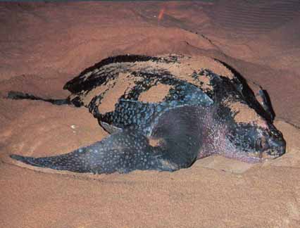
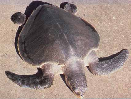
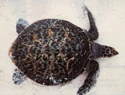
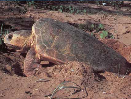
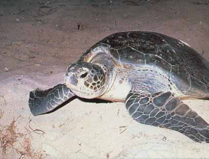
Standard Survey Methods
Appendix 7.12.1 Turtle identification sheet.
Marine Turtles found in the Red Sea and the Gulf of Aden.
Pictures courtesy of: Queensland Department of Environment and Heritage
Chelonia mydas (Green turtle)
Eretmochelys imbricata (Hawksbill turtle)
Lepidochelys olivacea (Olive ridley turtle)
Caretta caretta (Loggerhead turtle)
Dermochelys coriacea (Leatherback turtle)
236

---

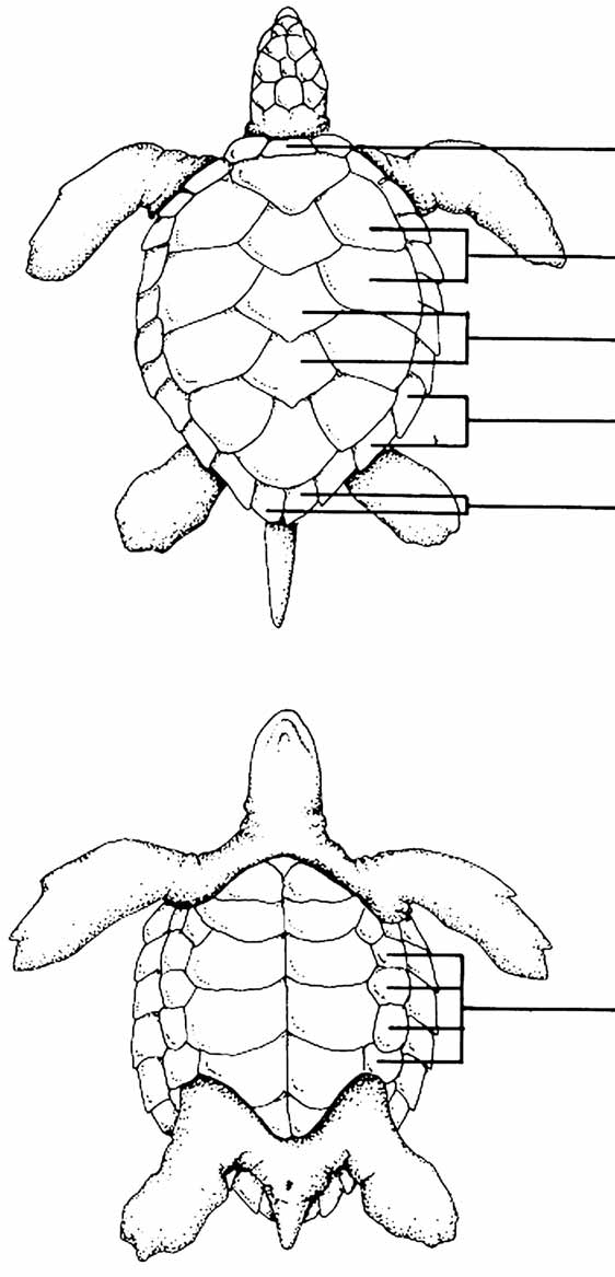
Marine Turtles
Description of key identifying characteristics (source: MILLER 1989).
CARAPACE
NUCHAL SCALE
LATERAL SCALES
CENTRAL SCALES
MARGINAL SCALES
POST CENTRAL SCALES
PLASTRON
INFRAMARGINAL SCALES
237

---

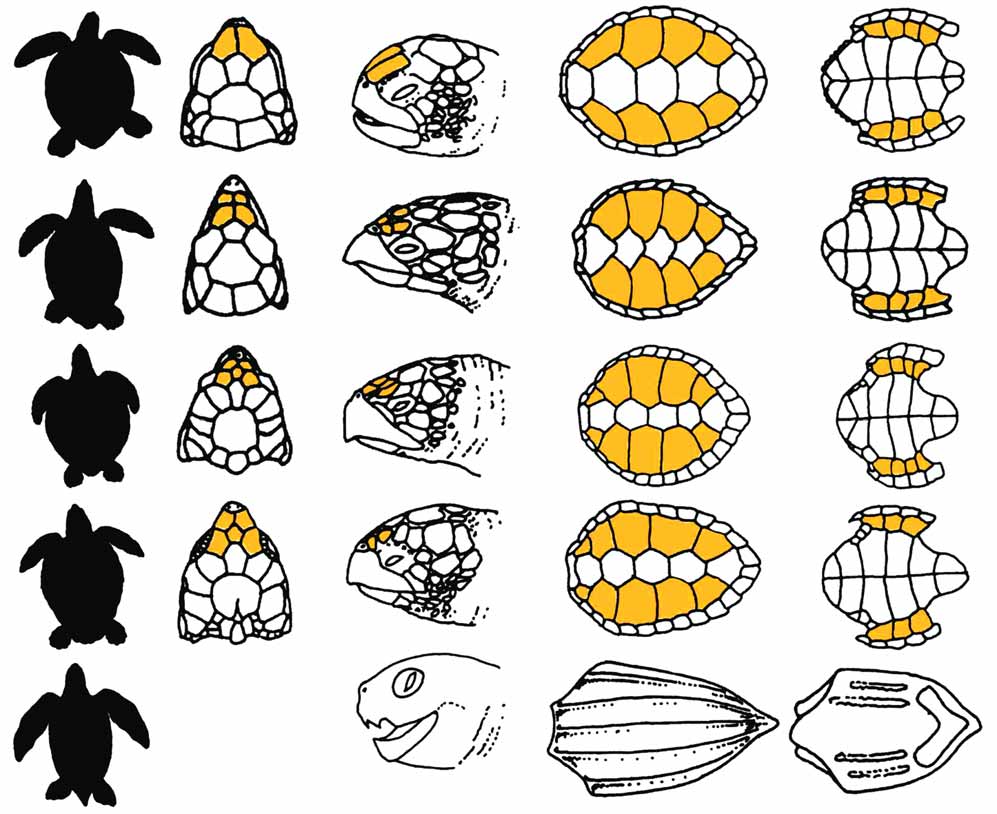
Standard Survey Methods
on
Plastr
et al. 1999.
T
Carapace
CKER
1989 and E
ILLER
M
Head (side)
Head (top)
.
Diagrams not to scale. Modified from
Silhouette
es
Plastron
without
ginal scutes with
prefrontal scutes.
a
, colour grey green.
ginal scutes
ginal scutes without pores.
a
Description
ginal scutes without pores.
a carett
een turtle)
Chelonia mydas
(Gr
Head with one pair prefrontal scutes.
Carapace with four lateral scutes, domed,
light to dark green and mottled.
with four inframar
pores.
Eretmochelys imbricat
(Hawksbill turtle)
Head with two pairs
Carapace with four lateral scutes, scutes
imbricated (overlapping). Plastron with four
inframar
Lepidochelys olivacea
(Olive ridley turtle)
Head with more than one pair of prefrontal
scutes. Carapace with five, six or more lateral
scutes, nearly circular
Plastron with four inframar
pores.
Carett
(Loggerhead turtle)
Head with more than one pair of prefrontal
scutes. Carapace with five lateral scutes,
longer than wide, colour red­brown. Plastron
with three inframar
Dermochelys coriacea
(Leatherback turtle)
Head with no scales. Carapace with five
distinct ridges and no scales.
Comparison of external featur
238

---

Marine Turtles
)
illing,
(Lo
ing, F
ay
) Olive Ridley

hambering, L
Notes
ights in Kg
e
WGT
























igging, C
) Loggerhead (Cc
All w
rack length
T
























.
ksbill (Ei
rack Width
T
andering, D
or cm
) Haw
TL
HW
merging, W
: E
PW
eturning
PL
Activity
R
Species: Green (Cm
All measurements in m
SCW
.
SCL
CCW
CCL
























Deformed
#
























Eggs
#
GPS Long:
























nesting beach surveys
Pits
#
























(Y/N)
Successful
























ctivity
A
























Sector
Beach
























New (Y/N)
GPS Lat:
























Species
























(24h)
ime
T
:

:

:

:

:

:

:

:

:

:

:

:

:

:

:

:

:

:

:

:

:

:

:

:

Tag #
Location: Site:
Date: Collector:
Data Sheet No:
.

.

.

.

.

.

.

.

.

.

.

.

.

.

.

.

.

.

.

.

.

.

.

.

Appendix 7.12.2 Sample data collection sheet for
239

---

Standard Survey Methods
Appendix 7.12.3 Sample data sheet for egg data collection.

Location: Site:
Date: Collector:
Nest Location:
GPS Lat:
GPS Long:
Nest #:
Species:
Data Sheet No:
Tag #:
Weight (g)
Diameter 1 (mm)
Diameter 2 (mm)
Mean Diameter (mm)







Standard
Deviation







Mean
Weight
(g)







Standard
Deviation





Appendix 7.12.4: Sample data sheet for hatchling data collection.
Location: Site:
Date: Collector:
Nest Location:
GPS Lat:
GPS Long:
Nest #:
Species:
Data Sheet No:
# Hatchlings Emerged:
Weight (g)
SCL (mm)
SCW (mm)
Mean Weight
Mean SCL
Mean SCW
(g)
(mm)
(mm)









Stand.
Stand.
Stand.
Deviation
Deviation
Deviation







































240

---

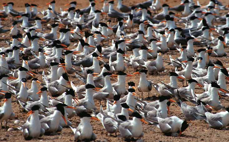
8
SEABIRDS
8.1 INTRODUCTION
The seabird populations of the Red Sea and Gulf of Aden
have been reviewed by COOPER et al. (1984), GALLAGHER et al.
(1984), EVANS (1987) and JENNINGS (1995). These works have
pulled together information from a wide variety of sources
covering a fairly long time span. In the first two papers, the
authors have attempted to estimate approximate population
sizes, or orders of magnitude for some breeding species, thereby
indicating the potential importance of the Red Sea and Gulf of
Aden (RSGA) region in an international context.
However, closer scrutiny of the above reviews shows that
little systematic survey work has been done on breeding seabirds
in the region. There are a few exceptions where whole
archipelagos have been covered, or national waters surveyed in
their entirety (Table 8.1). Some works on avifauna have given
estimates of national population sizes and breeding seasons for
some of the more frequently encountered species. However,
even where systematic surveys have been undertaken, there has
been little use of a systematic methodology. The importance of
the RSGA region for seabirds is not in doubt. Several endemic
taxa occur, including the white-eyed gull Larus leucophthalmus,
red-billed tropicbird Phaeton aethereus indicus, spoonbill
Platalea leucorodia archeri and the brown noddy Anous stolidus
241

---

Standard Survey Methods
plumbeigularus. A further group of taxa, at
conservation agencies, and amateur
both specific and sub-specific level, is
volunteers organised by the Seabird Group
endemic to the NW Indian Ocean area.
covered virtually all known coastal seabird
Important sub-populations of many of these
colonies, using standardised but flexible
taxa breed in the RSGA region. Species
methodology. Subsequently, a book was
include the Jouanin's petrel Bulweria fallax,
published (CRAMP et al. 1975), which
Socotra cormorant Phalacrocorax
summarised much of the numerical and
nigrogularis, sooty gull Larus hemprichii,
distributional data in annotated maps.
swift tern Sterna bergii velox and white-
Relative colony size and species accounts
cheeked tern Sterna repressa.
were shown using administrative counties as
the geographical unit for totals of pairs or
individuals. A hard copy file of raw counts for
A brief review of the development of
each colony, island or coastal section was
seabird survey methods in Europe puts this
deposited in national libraries and amongst all
work in context. The NE Atlantic is an
organisations that assisted with the
important area for breeding seabirds and there
coordination of the Operation Seafarer survey.
is a long history (30 years) of seabird
Fifteen years later, a slightly more rigorous
monitoring. The baseline survey, Operation
methodology was proposed for a re-survey,
Seafarer, was undertaken in 1969­70.
the Seabird Colony Register (SCR), which
Professional ornithologists employed by
was undertaken between 1985­87. Again a
Country National
avifauna:
Important recent seabird studies:
Name of archipelago
atlas (A); list (B)
whole country (A); archipelago
(B); single species in large area (C)
Egypt GOODMAN &
JENNINGS et al. 1985 (B)
Islands off Hurghada and
MEININGER 1989 (A)

much of Gulf of Suez


HOATH et al. 1997 (B)
Mouth of Gulf of Suez


FRAZIER et al. 1984 (A)

Jordan ANDREWS 1995 (B)



SHIRIHAI et al. 1999


(B)
Saudi
JENNINGS 1995 (A)
ORMOND et al. 1984 (A)

Arabia


NEWTON & SUHAIBANY 1996 (A)



GOLDSPINK et al. 1995 (B)
Farasan


JENNINGS 1988 (B)
Farasan


SYMENS 1988a (B)
Farasan


NEWTON & SYMENS 1996 (C)

Sudan NIKOLAUS 1987 (A)
MOORE & BALZAROTTI 1983 (B)
Suakin & Mohd. Qol
Eritrea SMITH 1951 (B)
CLAPHAM 1964 (B)
Dahlac
Yemen JENNINGS 1995 (A)
EVANS 1989 (B)
Al Luhayyah

BROOKS et al. 1987 (B)
PORTER & AL-SAGHIER 1998 (B)
Al Hudaydah

PORTER et al. 1996 (B)


Djibouti WELCH & WELCH 1984

(B)
Somalia ASH & MISKELL 1998
NORTH 1946 (B)
Mait Island
(A)
Socotra KIRWAN et al. 1996 (B)



Table 8.1 Sources of information regarding seabird numbers and distribution in the RSGA region.
242

---

Seabirds
book was published, LLOYD et al. (1991). This
During the early 1990's, several RSGA
provided a critique of discrepancies between
countries and others in Arabia began to
the two surveys, in the light of the different
contribute counts of wintering waterfowl to
methodologies used for different groups of
the International Waterfowl Census, organised
species. The major difference between the two
by the International Wetlands Research
surveys was that the principal output of the
Bureau (now Wetlands International). Within
SCR was a computer database. This has been
Saudi Arabia, only relatively small sections of
updated annually for a sample of colonies that
the Red Sea coastline could be covered by
are monitored regularly as part of the Seabird
ground counts. However, the availability of
Monitoring Programme (SMP).
light aircraft used for protected area patrols
with the National Commission for Wildlife
Conservation and Development (NCWCD)
WALSH et al. (1995) have produced a very
enabled much larger areas to be covered from
comprehensive manual of suitable
the air. This aerial survey work was usually
methodologies, that covers basic census and
undertaken in January/February outside the
more intensive productivity monitoring.
main breeding season for seabirds. However,
There is now much greater use of standardised
it soon became apparent that some species
methodologies and these are presently being
were nesting in the winter on some inshore
used in a third census of all colonies in Britain
islands, e.g. pink-backed pelican Pelecanus
and Ireland called Seabird 2000.
rufescens, brown booby Sula leucogaster and
Caspian tern Sterna caspia. With practice,
methods and routes were refined so that these
Surveys in the RSGA region and
species and their nests could be counted.
elsewhere in the Middle East prior to the
Subsequently, the numbers and distribution of
1990's were typically done during brief,
pelicans especially, became better known
opportunistic `walk-around' visits. However,
(NEWTON & SYMENS 1996). The next logical
the Gulf War of 1991 and the ensuing serious
step was to expand aerial coverage to summer
oil pollution in the northern Arabian Gulf
breeding seabirds and in 1993 a full aerial
(EVANS et al. 1993) changed the course of
survey of the Farasan archipelago was
seabird studies in the region. An
undertaken (GOLDSPINK et al. 1995). ground-
environmental disaster can act as a stimulant
truthing was also done to assess the accuracy
for improved monitoring and protection of the
of the aerial counts. Following extensive
marine environment. Detailed research
planning, a survey of all other Saudi Arabian
carried out on the Saudi Arabian Gulf islands
Red Sea islands was completed in summer
between 1991 and 1995 has resulted in refined
1996, together with a re-survey of some of the
methodologies for the census of summer
Farasan Islands (NEWTON & AL SUHAIBANY
nesting terns (SYMENS & EVANS 1993;
1996a, 1996b). Thus, work completed in the
SYMENS & AL SUHAIBANY 1996) and winter
Arabian Gulf and Saudi Red Sea has resulted
breeding Socotra cormorants (SYMENS et al.
in a variety of suitable methods being
1993; SYMENS & WERNER 1996). All tern
developed. Their application to the wider
species monitored in the Gulf are also
RSGA region is pertinent. However, for some
breeding in the RSGA region and the methods
species we are still woefully short of
are directly applicable. The Socotra area itself
information on the precise timing of nesting
is fairly peripheral in the breeding range of
seasons and whether these vary from year to
Socotra cormorants, though small numbers
year. For petrels (Procellariidae), which only
may nest near the coast of Yemen and survey
visit their colonies during the hours of
methods given in SYMENS & WERNER (1996)
darkness, we also lack an understanding of
would be appropriate.
nesting habitat.
243

---

Standard Survey Methods
8.1.1 Definitions
February and late April, and include Caspian
tern, Saunder's tern Sterna saundersi, herons
True seabirds:
and spoonbills. Some species such as the
Typically defined for the RSGA region as
brown booby have been found at nests in most
members of the following families, which are
months of the year. This situation could arise
dependent on the marine environment for the
for several reasons. Timing may vary in
whole of the annual cycle: petrels and
response to prey abundance in different areas
shearwaters, tropicbirds, boobies, cormorants,
at different times. Nesting could occur at sub-
gulls and terns.
annual intervals. Finally, there may be several
nesting "waves" at particular colonies, with
more experienced breeders commencing
Other seabirds:
earliest and less experienced pairs later. Only
Those families associated with the marine
regular visits to key sites over a period of
environment for the breeding season and
several years will throw light on this situation.
typically for much of the annual cycle:
pelicans, some herons and egrets, spoonbills.
These guidelines propose a framework for
the collection of information on breeding
Raptors and waders:
seabirds from countries bordering the Red Sea
Osprey Pandion haliaetus and crab plover
and Gulf of Aden.
Dromas ardeola are representatives for each
group that are dependent on the marine
environment in the RSGA. Although sooty
The specific aims for each country should
falcons Falco concolor nesting in the RSGA
include:
region utilise marine islands, their food base
typically consists of migrant passerine and
Production of a national inventory of
near-passerine birds. Additionally, many
seabird colonies in which the
Kentish plover Charadrius alexandrinus nest
following topics are covered:
on mainland beaches and islands and utilise
intertidal areas for feeding on invertebrates;
species present, breeding status,
some also nest inland around freshwater, the
number of pairs (or individuals),
margins of rivers, lakes and reservoirs.
habitats utilised;
size, topography and habitats of
each island/colony;
8.1.2 Breeding Seasons
timing of nesting or occupation of
Three seasons are referred to in the
islands/colonies;
following text; the commencement of a
season is marked by egg laying. Summer
human activities on or around each
breeders refer to those species that appear to
island/colony, direct and indirect
lay principally in late May to July (most
threats to seabirds;
terns). Winter breeders, including Socotra
cormorant, pink-backed pelican and osprey,
conservation actions needed,
may initiate clutches from the autumn
especially where human
(October) onwards, but the former species
occupation has been noted or
may nest in "waves", over a protracted period.
sensitive species are present.
Spring breeders are those that lay between
244

---

Seabirds
An estimate of geographical (regional)
Maps
population sizes and an evaluation of
The following maps are usually
the relative importance of sites. Those
sufficiently accurate and identify most
holding 5% or more of the
permanent islands:
biogeographical population may be
considered of international
British Admiralty Navigation Charts
importance. Such criteria for seabirds
or other local equivalents
differ from RAMSAR Convention
regulations, where sites holding 1% of
UK Ministry of Defence including:
a biogeographical population or
20,000 waterfowl are considered
Operational Navigation Charts (ONC)
internationally important.
Series 1:1,000,000, for example,
Production of a Conservation Action
ONC H­5 North Red Sea, Suez,
Plan which integrates seabird data
Aqaba
with other national/regional coastal
ONC J­6 Central Red Sea
initiatives towards the establishment
of marine protected areas (MPAs) and
ONC K­5 Southern Red Sea
the implementation of integrated
coastal zone management (ICZM)
ONC K­6 Gulf of Aden
strategies.
and:
The Tactical Pilotage Charts (TPC)
8.2 METHODS
Series at 1:500,000. Source: Air Force,
Airlines, smaller aircraft charter
companies.
8.2.1 Phase 1: Desktop Planning
The senior ornithologist in each country
The latter offer much more detail and are
should commence by preparing a list of all
perhaps the best for making initial lists of
islands in their territorial waters (Gulf of
islands. There are four sheets for each ONC,
Suez, Gulf of Aqaba, Red Sea, Gulf of Aden).
with alphabetic coding as follows: A =
All available maps, and perhaps satellite
northwest; B = northeast; C = southeast; D =
images, both hard copy and electronic, should
southwest. For example, sheet TPC J­6C
be scrutinised. In the RSGA region, virtually
covers the southeast part of ONC J­6 i.e. a
all seabird colonies are on islands, as they are
small part of the Red Sea coastline on the
free from the majority of terrestrial predators.
Saudi/Yemeni border.
However, remote sections of mainland coast
with sand spits are also relatively
inaccessible. Cliffs should be added to a
The Ministry of Petroleum & Mineral
reserve list to check as a second priority. Also,
Resources, Kingdom of Saudi Arabia (KSA),
mainland bays that harbour dense mangroves
produces some good maps at 1:500,000 scale.
often contain isolated stands that form small
Other countries probably have equivalent
islands without a solid substrate. These can be
maps produced by the national authority that
utilised by tree-nesting species such as
regulates oil exploration.
pelicans, herons and spoonbills. Again, add
such sites to the secondary site list.
245

---

Standard Survey Methods
The information extracted from maps
were typically brief `walk-around' visits, and
should be entered into an EXCEL type
population estimates are usually vague.
spreadsheet under the following headings:
However, one should be able to extract lists of
which species were present, those proven to
Name (real or geographically based,
be nesting, nesting habitat and a broad
e.g. island southeast of Jazirat One);
evaluation of numbers on an order of
note any alternatives in use.
magnitude scale:
Latitude (central point if large island)
A = 1­10 pairs,
Longitude (as above)
B = 11­100 pairs,
Approximate island size (three
C = 101­1,000 pairs,
categories: (A) small <500 m;
(B) medium 501­5,000 m; (C) large
D = 1,001­10,000 pairs and
>5,001 m, all measured along the
long axis)
E >10,000 pairs.
Any other details (presence of fishing
Again, such information can be entered on
villages, coastguard stations,
the EXCEL file as species; breeding (Yes / No);
mountains plus spot height etc.)
and order of magnitude (A­E).
The overall coastal zone should be
split into several sectors that may
Two lists of islands (derived from
eventually form reasonable field
historical and recent texts) should then be
survey units.
ranked in order of importance for breeding
seabirds.
Literature
Once the planning team is familiar with
the distribution and names of islands in
8.2.2 Phase 2: Resource Review
territorial waters, the ornithological literature
can be reviewed. Many general references to
Resources should be reviewed to assess
the RSGA region can be found in the 1990
availability under the following headings:
ALESCO­PERSGA bibliography edited by
personnel, transport, equipment, contacts and
MORCOS & VARLEY (pages 132­134 for birds)
liaison with other organisations.
and its companion volume containing
references for the period 1985­1998
(PERSGA/GEF 2002). More recent papers
Personnel
are listed at the end of this document.
List those personnel in your organisation
Literature should be classified under two
who can either participate in surveys, or act in
headings: historical (pre­1980) and recent
a support capacity in the field or in the data
(1980­2003). Experience has shown that the
analysis/presentation phase. Note their
situation described in recent papers is usually
ornithological skills on a three-point scale of
still applicable today, unless there have been
`some', `reasonable', `good' for the
significant military or tourist infrastructure
following: bird identification, bird census or
developments at the location in question.
counting experience, survey techniques
Information extracted from the literature
(knowledge of transects/quadrats), bird
should focus on the breeding status of species
ringing.
present at the time of the survey. Most surveys
246

---

Seabirds
Also record other skills that will be useful
Contacts and Liaison
in seabird surveys including boat handling,
Within your own organisation, liase with
ability to swim, navigation e.g. use of
other specialists (e.g. those working on turtles,
compass and GPS, knowledge of particular
marine mammals and mangroves) regarding
geographical areas, local contacts.
their survey programmes. Sharing transport or
survey flights is beneficial in reducing costs.
It is unlikely that many national organisers
have an abundance of experienced staff
Outside your own organisation, initiate
available. A training programme may need to
communication with a range of useful contacts
be considered.
(as above). In some instances you may be able
to recruit volunteer birdwatchers from natural
history societies who could assist in field
Transport
surveys. Identify all sites deemed sensitive for
The availability of vehicles, boats and
military or national security reasons; these
light aircraft needs to be assessed within your
should not be visited by field survey teams.
own organisation and within others that may
be able to assist you in reaching particular
islands. A useful exercise is to annotate
8.2.3 Phase 3: Fieldwork Options
coastal maps with the locations of coastguard
stations, navy bases, fisheries patrol
To produce a national seabird colony
vessels/bases, fishing villages, marinas and
inventory two main tasks have to be
pleasure boat moorings, marine research
accomplished:
centres and so on. Try and find out which
islands are covered by staff from these
A systematic reconnaissance (which
institutions and thereby identify gaps where
islands are used by seabirds, which
you will have to use your own boat or charter
species are present, whether they are
some alternative.
nesting) and
A more detailed monitoring of the
Equipment
more important, accessible, sites and
Relatively little scientific equipment is
colonies in which actual numbers may
required for basic seabird surveys other than
be assessed.
the usual binoculars, telescopes and tripods.
Waterproof notebooks or diving slates are
useful during very humid times of year. If
Aerial Survey
detailed nest counts are to be undertaken in
Both fixed-wing aircraft and helicopters
dense colonies, then a variety of light ropes
can be used to carry out aerial surveys.
(50 m in length) and tape measures will be
needed. GPS (with water tight `aquapac'
pouches to keep them dry), compasses and
Fixed-wing aircraft
other marine navigation and safety equipment
These are perhaps best for rapid
will be needed for offshore work and travel.
reconnaissance. In summer 1996, virtually all
The use of computers and data analysis
islands in the Saudi Red Sea were overflown
software is addressed at a later stage.
in a series of 12 missions (flights) that ranged
Generally speaking, use of laptop computers
in length from two to five hours flying time
in the field is not advisable owing to dust,
(NEWTON & AL SUHAIBANY 1996a). A basic
sand, humidity, etc.
procedure follows:
247

---

Standard Survey Methods
Discuss your rough itinerary with the
breeding birds tend to flush and
pilot several weeks in advance. The
disperse first, whereas those on nests
pilot will advise you as to restricted
with eggs and/or chicks are usually
areas, range and flying time with
most reluctant to fly off. Once bird
different numbers of observers etc.
counts have been made, if time and
Time will be needed to apply for and
fuel permit, make a further overpass to
receive approval of flight plans.
photograph dense colonies. Over
smaller islands (size classes A and B)
The day before your flight, give the
you should not spend more than 5
pilot a numbered list of coordinates for
minutes overhead, and often a lot less.
all islands/sites you wish to fly over on
Aerial surveys in summer should be
the next day. The pilot will enter these
confined to early morning
into the aircraft GPS and this will
(0600­1030) or late afternoon
relieve you of much navigational
(1500­1830) to minimise heat stress
responsibility during the flight so that
on adult birds or their eggs and chicks.
you can concentrate on identifying and
During winter, a longer part of the day
counting birds.
may be used.
Immediately prior to your flight (one
hour), take motion sickness pills if
Helicopters
necessary. Check you have all
These tend to be noisier, slower and
necessary maps and recording forms
probably cause more disturbance to nesting
plus sufficient drink and food (easy to
birds than fixed-wing aircraft. However they
eat in a confined space). Divide data
may be better as platforms for aerial
collection topics between the number
photography of dense colonies (e.g. Socotra
of observers you have (usually one to
cormorants, pink-backed pelicans), given
three). For example, one observer may
their ability to remain stationary. The
record island information (size,
helicopter should not fly too low as the
substrate, signs of human occupation,
downdraft from the rotors can blow eggs and
habitats etc.) and the other(s) record
chicks out of their nests. See SYMENS &
bird counts. The most experienced
WERNER (1996) for more details.
person should do the latter.
Once airborne over the sea in your
Boat Survey
target area, fly at 100­300 feet
Boats will usually be used to gain access
(30­90 m) above sea level as slowly
to islands. Larger and faster boats are better
as possible (probably about 90 knots).
for access to more remote offshore or distant
Usually, several overpasses of each
locations. An inflatable dingy with outboard
island will be required to cover the
engine may be needed to land on many islands
range of species. If two bird counters
with barrier reefs. During crossings of open
are present, split the species, or one
sea, try and maintain watch for seabirds,
count nests and the other birds. In the
particularly petrels and shearwaters. This may
first few surveys, try and evaluate
be the only opportunity to discover which
which species flush first and disperse
nocturnal or burrow-nesting species are
furthest on approach by the aircraft
present in your area, as they will not be seen
and those which stay together for
during daylight visits to islands. In some
longer in more detectable flocks.
instances, it may not be feasible to land, and a
Several overpasses are often necessary
boat circuit of the island may be your only
to flush species that nest under thick
opportunity to see which species are present.
cover, e.g. brown boobies. Non-
248

---

Seabirds
Landing may be prevented if the sea state is
Class C­size islands
too rough, if the island is totally surrounded
Islands of this size may have permanent
by impenetrable reef or inaccessible cliffs or
human settlements of one sort or another in
if you simply have insufficient time. For small
which case vehicles may be available to move
(Class A) islands, a sea circuit may provide
about the island (e.g. Farasan Kebir and Segid
enough information. It may be necessary to
in the southern Saudi Red Sea or Dahlac
count cliff-nesting species such as tropicbirds.
Kebir in Eritrea). However, it is also likely
If a prior aerial reconnaissance has not been
that cats, rats and mongooses will be present
done, a boat circuit can be useful to indicate
and large seabird colonies are improbable. For
presence and distribution of habitats and
example, the only seabirds nesting on Farasan
species to help plan a strategy once you are on
Kebir away from tall, dense stands of
the ground. Some nesting species, e.g. brown
mangrove are a couple of small Saunder's tern
boobies, should not be approached closely
colonies on more remote sandy beaches or
during the incubation and early chick stages
headlands. It may require several days to
as they are unable to defend their nests from
cover such islands adequately.
marauding white-eyed or sooty gulls, which
are usually present around the periphery of
colonies.
The following sections describe methods
appropriate to all species known to nest in the
RSGA region. However, some basic
Landing on Islands
methodologies are common to various species
Both the time available and the size of
groups, or habitats, and will help in the rapid
island are pivotal in deciding how to conduct
assessment of islands if time is limited.
the survey. Often some spells of careful
observation from higher vantage points may
be a better use of time than a mad rush to walk
8.2.4 Terrestrial Methods
to each corner of the island or around its
perimeter.
Most methods require an estimation of
nest densities in different habitats and then the
extrapolation of densities to the approximate
Class A­size islands
area of the island covered by that habitat type.
Plan to spend about two hours on land for
Prior awareness of the types of situations in
a rapid assessment, as long as your presence is
which various species nest and colony types
not continually disturbing all nesting birds on
will help in allocating search effort. Two
the island. All areas can be reached on foot
slightly different approaches are needed to
and even mangrove stands or dense shrubbery
determine the potential number of nesting
can be checked.
seabirds, depending on whether they are semi-
colonial or colonial. For the former, e.g.
bridled terns, vantage points need to be
Class B­size islands
located and counts made after the birds have
Allow eight hours, i.e. all day, and try and
resettled. If counts are conducted during
pick a day with some cloud cover, so that
incubation, note that one member of a pair
personal exhaustion and dehydration do not
incubates while the second frequently perches
influence your results.
above the nest on the top of a bush. Thus, the
total number of perched birds approximates
the number of pairs in the area. In more
compact colonies, e.g. white-eyed gulls and
white-cheeked terns, it is necessary for two
249

---

Standard Survey Methods
observers to walk in parallel three to five
Tree nesters, usually on canopy, e.g.
metres apart and record the number of nests
pink-backed pelican, spoonbill, cattle
and clutch sizes. The following descriptions
egret Bubulcus ibis.
give examples of habitats in which dispersed,
semi-colonial and colonial species are found.
8.2.5 Ringing
Bird ringing is a widely used tool in
Dispersed species
ornithological monitoring studies. In general,
Territorial, e.g. osprey, possibly
ringing does not have a significant role in
goliath heron, Ardea goliath, and
standard surveys aimed at assessing
purple heron, A. purpurea, (but in
population size. The key information to be
dense mangrove).
gained from ringing concerns the survival and
mortality rate, longevity, breeding site
Scarce habitats, e.g. red-billed
fidelity, and distribution patterns for birds
tropicbird in caves/niches, in cliffs or
using the RSGA region in, or out of, the
fossil coral overhangs.
breeding season. As adults, seabirds are not
easy to catch, given their normal habit of
Semi-colonial or loosely colonial species
nesting in open habitats. Thus, most seabird
(may cover whole island)
ringing involves catching and marking pre-
Ground nesters, e.g. Caspian tern,
fledging chicks; large numbers can be ringed
Saunder's tern, brown booby, sooty
relatively quickly in nesting colonies.
gull (usually beside or under some
However, seabirds are usually long-lived and
cover).
do not return to breeding areas for several
years. Information is gained from the use of
Under light vegetation, e.g. bridled
standard metal rings only when the individual
tern, also under overhangs in fossil
is recovered, i.e. found dead or deliberately
coral.
killed, or re-trapped. Use of field readable
Sub-colony, in or under medium
colour rings increases the likelihood of
height vegetation, e.g. little green
detecting ringed birds. A single colour can be
heron Butorides striatus, western reef
used to indicate chicks ringed in a particular
heron Egretta gularis, and brown
year or location (colony or island).
noddy.
Colonial species (usually discrete entities
Chick ringing can be used in intensive,
covering relatively small parts of island)
single site based studies to give information
Ground nesters, very compact
on survival and fledging rates. It can also be
colonies, large numbers, e.g. swift and
used in mark-recapture studies that indicate
lesser-crested terns Sterna bengalensis,
efficiency in finding chicks for species that
Socotra cormorant.
tend to hide in vegetation.
Ground nesters, compact colonies but
inter-nest distances 1­5 m e.g. white-
Although ringing is not a census tool, it is
cheeked tern, white-eyed gull.
always worth checking the legs of all dead
Underground nesters, usually in
birds found while doing fieldwork. Ring
dunes/berm or other sandy area, e.g.
recovery can yield important information
crab plover.
about the origins of birds in a colony.
250

---

Seabirds
8.2.6 Threats to Nesting Seabirds
persistent compared to closely related species
nesting in temperate or Arctic conditions.
The majority of seabirds nest in close
Terns also resettle relatively rapidly. Even so,
proximity to each other in colonies. This
the heat stress on eggs or small chicks
increases their overall vulnerability to
exposed during the middle of the day is
disturbance from human visitors or predators.
potentially very damaging. For some larger
When visiting seabird islands, one should
species, being forced to leave their nests can
always be aware of the disturbance being
give sufficient time for predators to steal eggs
caused and try to minimise the impact of the
or chicks. This has been observed for brown
visit. However, while on islands collect as
boobies: in flight over land, the adults are not
much information as possible, not only on the
very manoeuvrable and have difficulty in
birds themselves but also on human uses and
returning to their nests, thus allowing sooty,
their likely impact, and on predator presence
and possibly also white-eyed, gulls time to
or absence. If you are present in an
steal eggs. Once chicks are able to move
archipelago for several days, talk to as many
independently, disturbance may cause them to
local inhabitants as possible, especially
break cover and walk or run out of their natal
coastguards and fishermen, and assemble a
territory where they become vulnerable to
short log-sheet of useful information to
harassment and sometimes predation by
supplement your own observations.
neighbouring conspecifics (observed in sooty
gulls). Sometimes parents of such displaced
chicks may fail to relocate them, or feed them,
Factors threatening the well-being of
once they are away from their own nests.
breeding seabirds are numerous and include oil
pollution, overexploitation of fish stocks and
habitat destruction (e.g. from development or
Human Exploitation
overgrazing of mangroves, see EVANS 1987).
This can take one of two forms: collection
and consumption of eggs, or chicks. Currently
the latter does not appear to be a problem in
Human Disturbance
the Red Sea region, though it is, or has been,
Casual human visits to breeding islands
a traditional activity elsewhere especially at
can cause significant disturbance to nesting
Socotra cormorant colonies in the Arabian
birds even if there is no deliberate
Gulf and off southern Oman. Anecdotal
interference. In many areas, access to islands
evidence can be collected from local towns,
is under the control of the local coastguards.
which may indicate if food exploitation is
Landing may be forbidden, except on
taking place presently or has in the past. The
designated islands where overnight shelters
collection of eggs of tropical seabirds,
and "temporary" camps are sometimes
particularly terns, is a widespread
established. However, rules and regulations
phenomenon in the Indian Ocean, Red Sea
are seldom rigidly adhered to, and
and Arabian Gulf. Based on experience in the
undesignated islands can often become
Farasan and Al Wajh archipelagos, Saudi
popular breakfasting and meeting places
Arabia, it is often difficult to ascertain how
amongst fishermen; disturbance is caused
deliberate or planned egg collecting is, or
when they search for firewood etc.
whether it is mainly opportunistic. Egg
collecting is not restricted to fishermen or
local villagers, but can also be carried out by
Small agile species such as terns respond
government officials. If egg collecting takes
swiftly to intruders, though their mobbing
place early in the nesting cycle it may have
response is much reduced and not as
relatively little impact as the birds have
251

---

Standard Survey Methods
sufficient time to re-lay. However, repeated
Nests: vacated or contents not visible
collecting may have a severe impact on the
and present breeding status thus
distribution and overall breeding success of
indeterminate.
terns, with long-term consequences at the
population level. Egg collectors leave a trail
of footprints. These can easily be
Aerial Survey
distinguished from those of casual visitors,
Two approaches can be used in isolation or
particularly when they move between and
in combination: direct counts and aerial
around vegetation patches systematically
photography. If sufficient personnel are
looking for bridled tern nests, or they link a
airborne or if the area to be covered is relatively
chain of empty white-cheeked tern scrapes.
small, using both is preferable. Photography is
most appropriate if personnel are relatively
inexperienced, although learning to make rapid
Introduced Predators
but approximate estimates is a valuable skill to
Cats are often deliberately brought to new
acquire. Films can be lost by developers or may
human settlements on offshore islands, such
lack quality (poor exposure or focus). Tally
as fishing camps and coastguard stations, to
(clicker) counters are very useful. To speed up
control rodent populations. However, some
the process count in units of ten, or 50 if
introductions are no doubt accidental from
numbers are large. The present availability of
concealed ship borne animals. Cats soon
motor drives, rapid autofocus and zoom lenses
become feral and numbers can increase
has made aerial photography very easy and
rapidly, with waste human food and garbage
reliable. Choice of film type (slide versus print)
acting as a buffer against seasonally
is not important though if the latter are used,
fluctuating natural food supplies. The white-
then print size needs to be somewhat larger than
tailed mongoose (Ichneumia albicauda) is
standard (i.e. at least 30 x 20 cm). Using a
also present on some of the larger Red Sea
camera that prints date and time onto each shot
islands. These small carnivores have been
can save much writing whilst in the air.
shown to affect the breeding success of large
However you should always record notes of
species such as ospreys (FISHER, pers. comm.)
island, sub-section etc. on a film shot log that
and they may be the principal factor
can be crosschecked with the recorded
preventing ground nesting seabirds from
route/time log that the pilot or navigator will
using certain islands.
keep. Once back at base when the films have
been developed, procedures for analysis of
prints and slides are slightly different.
8.2.7 Census Techniques
Count Units
Prints
Make sure that count units and methods
Several good quality copies are made
are recorded on field sheets or notebooks. The
(generally enlargements, sometimes
following can be used as count units:
photocopies) and assembled into an
overlapping mosaic. An island colony is divided
Individuals: usually for non-breeding
into sub-sections drawn on the prints and each
birds or aerial counts where sub-
team member marks nests (cross or circle) with
canopy nest cannot be seen.
a fine pen. The exercise is repeated several
times and the average count used. Remember to
Occupied (adult present) or Active
include the count unit on your data sheet:
(egg or chick present) Nests: either
individual birds e.g. roosting cormorants;
from ground or aerial counts.
occupied or active nests; or vacated nests.
252

---

Seabirds
Slides
Flush Counts
Project slides onto large sheets of white
These can be used when the nesting birds
paper, where they can be marked in the same
(usually those incubating or with small
way as prints. It is usually more difficult to
chicks) rise up with reasonable synchronicity,
separate adjacent sub-colonies reliably on
and fly around above the colony in a relatively
slides, as they cannot be viewed
compact flock on approach by a human. It is
simultaneously.
especially useful for terns in medium to large
sized colonies. Always attempt counts, even if
you intend to walk into the colony to
Several useful papers review topics such as
undertake a nest count. The count unit is of
the comparability of print versus slide media
individual birds and the mean of several
and detailed counts versus estimates (e.g.
counts should be recorded. The relationship
REYNOLDS & BOOTH 1987), and between-
between the number of birds counted and the
observer variability in colony counts, for
number of pairs or nests present varies with
photographs (HARRIS & LLOYD 1977). Aerial
the stage of incubation and species. Validation
photographs provide good records of the
studies need to be conducted if it is necessary
actual location of colonies on particular
to convert individual counts to numbers of
islands and how they grow if the population is
pairs or nests. For example, BULLOCK &
increasing (e.g. HILL 1989). Photographic
GOMERSALL (1981) give a conversion factor of
records can also be very useful during
1.5 for temperate nesting common and arctic
subsequent ground visits.
terns during late incubation in Scotland. In
this case, a count of 100 individuals would be
eqivalent to 67 nests. SYMENS
&
Ground Counts
ALSUHAIBANY (1996) give similar information
The main ground count techniques used do
for white-cheeked and bridled terns nesting in
not require equipment other than binoculars or
the Arabian Gulf, although the conversion
telescopes and include: counts from vantage
factors may not be exactly replicable for the
points, flush counts, and walk-through counts.
RSGA region.
More time-consuming methods such as belt
transects (for terns) and quadrats (for terns and
cormorants) require some basic mapping and
Walk-though Counts
need ropes, tape measures, compass and
In small to medium sized tern or gull
bamboo canes (or similar) as markers.
colonies, walk-through counts can be
effective. Depending on nest density, two or
more observers walk in parallel through a
Vantage Points
colony, counting nests on either side within
This method requires the presence of
half the distance between the next person.
dunes or other slightly elevated terrain from
Tally counters are useful, especially if you are
which to observe the colony. Count the
recording clutch sizes or several species in the
number of occupied nests using binoculars or
same colony. If several passes through the
telescope. If the colony is fairly large, split it
colony are needed, then it can be useful to lay
into sections first, using landmarks that you
a rope through the colony to delimit the area
can relocate with ease. Suitably chosen
you have covered. On sandy substrates your
vantage points cause little disturbance but are
footprints can also be used to prevent double
best used for small to medium sized colonies.
counting.
Where birds are very densely packed or the
colony is very large, different sampling
procedures will have to be used.
253

---

Standard Survey Methods
An alternative technique, which does not
Counts of Nest Structures outside the
require in situ counting is as follows: enter the
Breeding Season
colony with a bag containing a sufficient
This method can be used for large Socotra
quantity of counted, dry, pasta pieces. Place
cormorant colonies, and perhaps swift and
one piece in each nest as proof that it has been
lesser-crested terns and brown boobies, when
counted. Once the colony is finished, subtract
the colony has been vacated. Nest scrapes,
the number of remaining pasta pieces from the
mounds or depressions can be identified and
initial total to get the number of nests. Do not
counted, or sampled by transects or quadrats.
use this method if large numbers of rodents
Counts may indicate the maximum number of
(mice or rats) are present on the island.
pairs that attempted to breed in the previous
season. SYMENS & WERNER (1996) give
details and limitations of this technique, but
Belt Transects
note that heavy rainfall may obliterate much
Belt transects are most suitable for species
evidence of nesting.
which do not nest at extremely high densities
such as white-cheeked tern and bridled tern.
Transects are conducted at regular intervals of
8.2.8 Methods for Species Breeding in
100­500 m parallel to the short axis across an
the RSGA region
island or colony. For each nest found, record
species, clutch size and location along the
The following section includes specific
transect. Also record total transect length. Use
details for individual species breeding in the
densities calculated from these data to
RSGA region. Where known, the habitats
estimate total populations for each island or
utilised, colony type and nesting season are
colony (see S
also given.
YMENS & EVANS 1993; SYMENS
& ALSUHAIBANY 1996).
Jouanin's petrel Bulweria fallax
Quadrats
Both swift and lesser-crested terns nest at
Area: Socotra and neighbouring islands.
extremely high densities. Belt transects right
through colonies would cause excessive
Habitat and colony type: Caves in coastal
disturbance. Instead make a lightweight frame
cliffs of soft limestone.
of rigid wire measuring 1 x 1 m. Lay this
carefully down at a selection of locations
Nesting season: Summer ­ autumn (eggs July,
evenly spread across the colony and count
fledglings November).
nests. The number of 1 m2 quadrats counted
will depend on the time available and colony
Appropriate methods: None described; the
size. Between ten and 30 should be adequate.
nesting cliffs are treacherous and inspection
While one person or team counts the nests,
would require competent rock climbers with
another should draw a map and measure the
ropes. Inspection of a sample of caves
size of the colony (at least the maximum
covering the range of sizes (depth, diameter of
length and breadth), so that the quadrat
entrance etc.) may yield a mean number of
density estimates, when averaged, can be
pairs per cave type. A colony size may then be
extrapolated to the area of the colony. This
estimated by multiplying the total number of
technique is particularly suitable during the
each cave type by the appropriate mean
incubation period.
number of pairs and summing them. An
alternative, or complementary approach
would be to classify the intensity of nocturnal
vocalisations at different cliffs or colonies and
254

---

Seabirds
allocate them to an index of probable nesting
Masked booby Sula dactylatra
population size. Such a method was
developed by RATCLIFFE et al. (2000) for Fea's
Area: Scarce; southern Red Sea, Gulf of
petrels in the Azores. This could be used as a
Aden.
suitable model, given nesting habitat of the
two species appears similar and equally
Habitat and colony type: Not well described;
inaccessible. On smaller islands with few or
rocky islands, possibly use trees on occasions.
no terrestrial predators, petrels may nest in
more accessible terrain. In this case, a tape
Nesting season: Summer ­ autumn?
playback methodology may be applied.
Appropriate methods: Direct count of nests
Relevant literature: TALEB 2002, RATCLIFFE et
from air, sea or vantage point.
al. 2000; [tape playback methodology is
described in JAMES & ROBERTSON 1985 for
Relevant literature: MORRIS 1962; NEWTON &
other Puffinus species and RATCLIFFE et al.
AL SUHAIBANY 1996b.
1998 for small petrels].
Brown booby Sula leucogaster
Persian shearwater Puffinus (lherminieri)
persicus
Area: Widespread, whole RSGA region.
This species has been discovered nesting on
Habitat and colony type: Very varied
Socotra in similar habitat to Jouanin's petrel.
including sandy beaches and islands, under
The above methods may therefore apply.
medium sized bushes, open rocky islands,
occasionally cliffs.
Red-billed tropicbird Phaethon
Nesting season: Very variable; possibly a
aethereus
prolonged season commencing in summer in
the south but with colonies active until
Area: Whole RSGA region.
January; in north may start earlier (possibly
April).
Habitat and colony type: Dispersed; holes and
crevices in cliffs.
Appropriate methods: Direct counts of nests
from air or vantage point. Do not disturb
Nesting season: Probably April to August,
colony during incubation as gulls will rapidly
possibly later in Gulf of Aden.
prey upon unguarded eggs.
Appropriate methods: Direct counts of
Relevant literature:
NEWTON
& AL
occupied holes, but usually can only be
SUHAIBANY 1996a; HOATH et al. 1997;
detected if bird seen entering or departing.
CLAPHAM 1964.
Adults flying around cliffs during the
probable nesting season may be an indication
of local breeding.
Relevant literature: HANSBRO & SARGEANT
2000; CLAPHAM 1964; NORTH 1946.
255

---

Standard Survey Methods
Socotra cormorant Phalacrocorax
but also in more isolated thickets of
nigrogularis
Euphorbia. Sometimes under nests of other
species (such as western reef heron,
Area: Islands off Yemeni coast in Gulf of
spoonbill), occasionally in holes and crevices
Aden.
in fossil coral.
Habitat and colony type: No recent
Nesting season:
Spring, probably
description in Gulf of Aden; usually large
commencing in March to April.
dense colonies on sandy or rocky substrate in
Arabian Gulf.
Appropriate methods: None known except
through searches of dense vegetation;
Nesting season: In Arabian Gulf, September
presence/absence possibly only data that can
to April with peak laying October to January.
be gathered.
Appropriate methods: Direct counts of nests
Relevant literature: NEWTON & AL SUHAIBANY
from a distance in colonies of size B to low
1996a; GOODMAN & MEININGER 1989.
D. For large colonies, high D to E, aerial
counts of "apparently occupied nests".
Cattle egret Bubulcus ibis
Relevant literature: SYMENS & WERNER 1996.
Area: Southern Red Sea.
Habitat and colony type: This species may
Pink-backed pelican Pelecanus rufescens
nest on nearshore islands in tall vegetation;
however, it does not utilise the marine
Area: Southern Red Sea.
environment as a food source.
Habitat and colony type: Usually on top of
Nesting season: Throughout the year, perhaps
tall mangroves Avicennia marina,
dependent on rains.
occasionally Rhizophora mucronata, or lower
bushes and exceptionally on the ground.
Appropriate methods: Direct nest counts of
small colonies; aerial counts for large
Nesting season: Winter, possibly November
colonies.
to March.
Relevant literature: JENNINGS 1995.
Appropriate methods: Direct counts from air
or aerial photographs, virtually impossible to
see nests from ground or sea level.
Western reef heron Egretta gularis
Relevant literature: N
Area: Whole RSGA region.
EWTON & SYMENS 1996.
Habitat and colony type: Usually small to
Little green heron Butorides striatus
medium colonies (A­B) in dense vegetation,
both mangroves and trees, often sub-canopy;
occasionally low cliffs.
Area: Widespread, whole RSGA region.
Nesting season: Spring ­ summer (March to
Habitat and colony type: Usually concealed in
August).
or under dense vegetation (e.g. mangroves)
256

---

Seabirds
Appropriate methods: None described;
Habitat and colony type: Usually small
thorough searches on foot of suitable habitat
colonies (B) on top of dense vegetation, both
on smaller islands.
mangroves and thickets, often associated with
western reef heron.
Relevant literature: JENNINGS 1995; NEWTON
& AL SUHAIBANY 1996a; GOODMAN &
Nesting season: Spring ­ summer.
MEININGER 1989.
Appropriate methods: Aerial counts, though
ground counts feasible if nesting in thickets of
Purple heron Ardea purpurea
medium height shrubs.
Area: Local, southern Red Sea.
Relevant literature: JENNINGS 1995; NEWTON
& AL SUHAIBANY 1996a; EVANS 1989.
Habitat and colony type: Probably dense
mangrove, unlikely to be colonial, compare
JENNINGS 1995.
Osprey Pandion haliaetus
Nesting season: Not known, possibly spring
Area: Widespread, whole RSGA region.
to summer.
Habitat and colony type: Usually well-
Appropriate methods: None described,
spaced, large nest structure in open situation,
thorough searches necessary to prove
found in all habitats though rarely directly in
breeding. Presence outside winter (April to
or on vegetation; occasionally semi-colonial.
August) may indicate local breeding.
Nesting season: Winter (November to April).
Relevant literature: JENNINGS 1995.
Appropriate methods: Easily detectable on
ground; aerial counts necessary to get
Goliath heron Ardea goliath
meaningful data from whole archipelago.
Area: Local, whole Red Sea.
Relevant literature: JENNINGS 1995; FISHER
1996.
Habitat and colony type: Usually areas with
plenty of mangrove; nests solitarily, sub-
canopy or on ground under cover.
Sooty falcon Falco concolor
Nesting season: Probably winter ­ spring.
Area: Scarce, whole length of Red Sea.
Appropriate methods: Thorough searches
Habitat and colony type: Variable, crevices or
necessary to prove breeding.
caves, on ground under mangroves.
Relevant literature:
NEWTON
& AL
Nesting season: Spring ­ summer.
SUHAIBANY 1996a.
Appropriate methods: Pairs usually flushed if
landings made on island; usually detectable
Spoonbill Platalea leucorodia
by aerial survey.
Area: Whole Red Sea, most common in south.
Relevant literature: GAUCHER et al. 1995.
257

---

Standard Survey Methods
Crab plover Dromas ardeola
Nesting season: Commences April/May in
north, June/July in south.
Area: Local along length of Red Sea.
Appropriate methods: Flush counts of adults
Habitat and colony type: Nests underground
emerging from nests can be made from air;
in burrows; in colonies (B­C) on sandy
loose colonies usually small, so nests can be
islands.
counted directly during ground work.
Nesting season: Summer (commencing
Relevant literature: JENNINGS 1995; NIKOLAUS
May/June).
1987; GOODMAN & MEININGER 1989; NEWTON
& AL SUHAIBANY 1996a.
Appropriate methods: Colonies can be quite
easy to overlook; direct counts of burrows
straightforward but not easy to prove
White-eyed gull Larus leucophthalmus
occupancy. If possible, do not walk through
colony, as burrows are very easy to collapse.
Area: Widespread, probably whole of RSGA
region.
Relevant literature: GOLDSPINK et al. 1995;
NIKOLAUS 1987; MORRIS 1992.
Habitat and colony type: Small colonies (B),
often in open sand, occasionally more rocky
substrate.
Kentish plover Charadrius alexandrinus
Nesting season:
Summer, probably
Area: Widespread, probably whole RSGA
commences June in north and July in south.
region.
Appropriate methods: As for sooty gull.
Habitat and colony type: Dispersed nests on
open shore just above high water mark in
Relevant literature: As for sooty gull.
seaweed, flotsam or broken coral rubble.
Nesting season: Spring, mostly February to
Caspian tern Sterna caspia
May.
Area: Widespread but scarce, probably whole
Appropriate methods: Nests difficult to find,
of RSGA region.
but adults frequently employ distraction
displays that are sufficient proof of breeding.
Habitat and colony type: Solitary or dispersed
loose colonies, usually fairly open sandy
Relevant literature: JENNINGS 1995.
areas. Occasionally nests on mainland coasts,
e.g. sand-spits.
Sooty gull Larus hemprichii
Nesting season: Spring, usually February to
April/May.
Area: Widespread, probably whole RSGA
region.
Appropriate methods: Nests can be detected
from air if few other species present;
Habitat and colony type: Dispersed or loose
otherwise detailed groundwork is needed.
colonies on both sandy and rocky islands.
Nests usually in shade of rock or small bush.
Relevant literature: JENNINGS 1995.
258

---

Seabirds
Swift and lesser-crested tern Sterna bergii,
should be taken not to trample eggs, as nests
S. bengalensis
can be quite cryptic. Flush counts of adults
attending nests are satisfactory if time limited.
Area: Widespread, whole of RSGA region.
Relevant literature: As swift tern, SIMMONS
Habitat and colony type: Large dense
1994.
colonies of both species often found side by
side; often on edge of larger sandy islands or
more centrally on smaller ones.
Bridled tern Sterna anaethetus
Nesting season: Summer, usually June to
Area: Common and widespread, whole RSGA
August, swift terns possibly earlier than
region.
lesser-crested terns.
Habitat and colony type: Colonies will often
Appropriate methods: Aerial counts can yield
stretch over whole islands with moderate to
acceptable estimates of numbers of
dense vegetation cover. Nests fairly well
individuals and nests; photographs could be
dispersed under bushes (although there may
useful for more accurate counts. Otherwise,
be more than one nest under any one bush) or
nest density needs to be measured in sample
small rocky overhangs.
quadrats or belt transects and extrapolated to
measured/estimated area covered by colony.
Nesting season: Summer, usually May/June to
August.
Relevant literature: SYMENS & AL SUHAIBANY
1996; SYMENS & EVANS 1993; NEWTON & AL
Appropriate methods: Numbers of adults
SUHAIBANY 1996a; MOORE & BALZAROTTI
flushed from nests can be estimated during
1983.
aerial counts. On the ground, counts of adults
perched on bushes following flushing during
the incubation period may give approximation
White-cheeked tern Sterna repressa
of numbers of pairs. If more detail required,
then sample quadrats or belt transects are
Area: Common and widespread, whole of
necessary. Make sure sampling covers the
RSGA region.
range of vegetation types, bush densities and
heights.
Habitat and colony type: Usually medium
sized (B to low C) colonies, frequently in
Relevant literature: As for swift tern, SWEET
open sandy areas or coral rubble; may be
1994.
several discrete sub-colonies even on quite
small islands.
Nesting season: Summer, usually June to
Sooty tern Sterna fuscata
August.
Area: Occasionally recorded breeding on the
Appropriate methods: Often difficult to detect
African coastline of the Gulf of Aden.
during aerial counts as colonies are amongst
larger numbers of bridled terns or brown
Habitat and colony type: In other parts of the
noddies. However, the number of nests can
world, nests in the open in very large dense
usually be counted by two or more observers
colonies similar to swift and lesser-crested
walking in parallel through a colony. Care
terns. However, colonies in RSGA region
probably relatively small.
259

---

Standard Survey Methods
Nesting season: Possibly June
Nesting season: Probably summer, May to
August.
Appropriate methods: Detailed methodology
given in paper below.
Appropriate methods:
Several aircraft
overpasses usually flush adults from
Relevant Literature: RATCLIFFE et al. 1999.
vegetation, although some adults may remain
in situ. However, aerial counts are probably
easier to undertake than ground counts, as it is
Saunder's tern Sterna saundersi
very difficult to count nests in dense
vegetation. More validation work urgently
Area: Widespread but local on Arabian side of
required on this species.
the Red Sea, apparently scarcer on the African
side.
Relevant literature: MOORE & BALZAROTTI
1983; NEWTON & AL SUHAIBANY 1996a.
Habitat and colony type: Small loose colonies
(A­B) in sandy areas; may nest on mainland
coasts.
8.3 DATA ANALYSIS AND
PRESENTATION
Nesting season: Spring, first eggs usually
April.
All field data should be transcribed onto
Appropriate methods: Very seldom detected
clean sheets as soon as possible after surveys
during aerial surveys; detailed ground work
are completed, then entered into EXCEL
needed to prove presence of nests.
spreadsheets on return to base camp. Two
formats can be used; the first covering
Relevant literature: JENNINGS 1995.
information on the islands themselves, and a
second giving bird and nest counts (see
Appendix 8.5.1). Suggested formats are
Brown noddy Anous stolidus
provided below.
Area: Widespread, southern Red Sea and Gulf
of Aden, usually on islands well offshore
The island and bird spreadsheets can be
(>20 km).
copied into a relational database such as
ORACLE or MICROSOFT ACCESS. Linked and
Habitat and colony type: Colonies usually
composite tables can then be generated and
large (C­D) on well-vegetated islands often
analysed. The data can then be imported into
covered with Suaeda fruticosa; rarely
a mapping package (e.g. DMAP or a GIS such
mangrove Avicennia marina. Nests sub-
as ARCVIEW).
canopy on branches of trees or bushes.
260

---

Seabirds
8.4 REFERENCES
FISHER, P.R. 1996. A report to the National
Commission for Wildlife Conservation and
A
Development on the status of the Farasan
NDREWS, I.J. 1995. The Birds of the
Hashemite Kingdom of Jordan. Andrews,
Islands Osprey Pandion haliaetus, Red Sea.
Musselburgh.
The Manchester Metropolitan University,
England. 57 pp.
ASH, J.S. & MISKELL, J.E. 1998. Birds of.
Somalia. Pica Press, Mountfield, UK. 336
FRAZIER, J.G., SALAS, S.S. & SALEH, M.A.
PP.
1984. Ornithological observations along the
B
Egyptian Red Sea coast, spring 1982: with
ROOKS, D.J., EVANS, M.I., MARTINS, R.P. &
P
notes on migratory and breeding species.
ORTER, R.F. 1987. The status of birds in
North Yemen and the records of OSME
Courser 1: 17­27.
Expedition in autumn 1985. Sandgrouse
9: 4­66.
GALLAGHER, M.D., SCOTT, D.A., ORMOND,
R.F.G., CONNOR, R.J. & JENNINGS, M.C. 1984.
B
The distribution and conservation of seabirds
ULLOCK, I.D. & GOMERSALL, C.H. 1981. The
breeding populations of terns in Orkney and
breeding on the coasts and islands of Iran and
Shetland in 1980. Bird Study 28: 187­200.
Arabia.
ICBP
Technical Publication
No.2: 421­456.
CLAPHAM, C.S. 1964. The birds of the Dahlac
Archipelago. Ibis 106: 376­388.
GAUCHER, P., THIOLLAY, J.M. & EICHAKER, X.
1995. The Sooty Falcon Falco concolor on
C
the Red Sea coast of Saudi Arabia:
OOPER, J., WILLIAMS, A.J. & BRITTON, P.L.
1984. Distribution, population sizes and
distribution, numbers and conservation. Ibis
conservation of breeding seabirds in the
137: 29­34.
Afrotropical region. ICBP
Technical
Publication No.2: 403­419.
GOLDSPINK, C.R., MORGAN, D.H., SIMMONS,
D., SWEET, G. & TATWANY, H. 1995. The
C
distribution and status of seabirds on the
RAMP, S., BOURNE, W.R.P. & SAUNDERS, D.
1975. The Seabirds of Britain and Ireland.
Farasan Islands, Red Sea, Saudi Arabia with
Collins, London. 287 pp.
a note on the possible effects of egg predation.
NCWCD/Manchester Metropolitan University
E
Report.
VANS, M. 1989. Breeding birds on some Red
Sea islands off North Yemen. Ornithological
Society of the Middle East Bulletin 23: 14­20.
GOODMAN, S.M. & MEININGER, P.L. 1989. The
Birds of Egypt. Oxford University Press.
E
551 pp.
VANS, M.I., SYMENS, P. & PILCHER, C.W.T.
1993. Short-term damage to coastal bird
populations in Saudi Arabia and Kuwait
HANSBRO, P. & SARGEANT, D. 2000.
following the 1991 Gulf War marine
Interesting ornithological observations from
pollution. Marine Pollution Bulletin
Yemen in spring 1998. Sandgrouse 22: 71­74.
27: 157­161.
HARRIS, M.P. & LLOYD, C.S. 1977. Variations
E
in counts of seabirds from photographs.
VANS, P.G.H. 1987. Seabirds of the Red Sea.
In: Key Environments: Red Sea. (Edwards,
British Birds 70: 200­205.
A.J. & Head, S.M. eds): 315­338. Pergamon
Press, Oxford.
261

---

Standard Survey Methods
HILL, M.G. 1989. The Alderney Gannetries ­
MORRIS, R.O. 1962. Two visits to the
photographic counts of Ortac and Les Etacs,
Haycocks (Hanish Islands, southern Red Sea).
Channel Islands, 1979­1989. Seabird
Sea Swallow 15: 56­58.
12: 45­52.
MORRIS, R.P. 1992. Observations on a colony
HOATH, R., RUSSELL, D., KHALIL, R. &
of Crab Plovers Dromas ardeola in Abu Dhabi.
KHALIL, D. 1997. The birds of the islands at
Sandgrouse 14: 34­47.
the mouth of the Gulf of Suez, Egyptian Red
Sea. Sandgrouse 19: 22­29.
NEWTON, S.F. & AL SUHAIBANI, A.H. 1996a.
Distribution and abundance of summer
JAMES, P.C. & ROBERTSON, H.A. 1985. The
breeding seabirds in the Saudi Arabian Red
use of playback recordings to detect and
Sea in 1996. Unpublished report. NCWCD,
census nocturnal burrowing seabirds. Seabird.
Riyadh. 56 pp.
8: 18­20.
NEWTON, S.F. & AL SUHAIBANI, A.H. 1996b.
JENNINGS, M.C. 1988. A note on the birds of
Survey of summer breeding seabirds in the
the Farasan Islands, Red Sea, Saudi Arabia.
Saudi Arabian Red Sea. Phoenix 13: 5­6.
Fauna of Saudi Arabia 9: 457­467.
NEWTON, S.F. & SYMENS, P. 1996. The status of
JENNINGS, M.C. 1995. An Interim Atlas of the
the Pink-backed Pelican (Pelecanus rufescens)
Breeding Birds of Arabia. NCWCD, Riyadh.
and Great White Pelican (P. onocrotalus) in the
134 pp.
Red Sea: The importance of Saudi Arabia.
Colonial Waterbirds 19: 56­64.
JENNINGS, M.C., HEATHCOATE, P.C., PARR, D.
& BAHA EL DIN, S.M. 1985. Ornithological
NIKOLAUS, G. 1987. Distribution atlas of
survey of the Ras Dib area and the islands at
Sudan's birds with notes on habitat and status.
the mouth of the Gulf of Suez, Egypt. Oil
Bonner Zoologische Monographien No.
Pollution Research Unit, Pembroke.
25: 1­322.
KIRWAN, G.M., MARTINS, R.P, MORTON, K.M.
NORTH, M.E.W. 1946. Mait Island ­ a bird-
& SHOWLER, D.A. 1996. The status of birds in
rock in the Gulf of Aden. Ibis 88: 478­502.
Socotra and `Abd Al-Kuri and the records of
the OSME survey in spring 1993. Sandgrouse
ORMOND, R., SHEPHERD, A.D., PRICE, A. &
17: 83­101.
PITTS, R. 1984. Sea and shore birds. In: Saudi
Arabian Marine Conservation Programme
LLOYD, C.S., TASKER, M.L. & PARTRIDGE, K.
Report No.4, Part 2. pp 124­140. University of
1991. The Status of Seabirds in Britain and.
York, U.K.
Ireland. T. & AD Poyser, London. 355 pp.
PERSGA/GEF 2002. A Bibliography of
MOORE, R.J & BALZAROTTI, M.A. 1983.
Oceanographic and Marine Environmental
Observations of sea birds nesting on islands of
Research 1985­1998. Red Sea and Gulf of
the Sudanese Red Sea. Bulletin of the British
Aden Region. PERSGA Technical Series
Ornithological Club 103: 65­71.
No. 2. PERSGA, Jeddah. 230 pp.
MORCOS, S.A. & VARLEY, A. eds. 1990. Red
PORTER, R.F., MARTINS, R.P., SHAW, K.D. &
Sea, Gulf of Aden and Suez Canal. A
SORENSON, U. 1996. The status of non-
Bibliography on Oceanography and Marine
passerines in southern Yemen and the records
Environmental Research. ALESCO/PERSGA
of the OSME survey in spring 1993.
and UNESCO. 198 pp.
Sandgrouse 17: 22­53.
262

---

Seabirds
PORTER, R.F. & AL-SAGHIER, O. 1998. The
SYMENS, P. & ALSUHAIBANY, A.H. 1996. Status
birds of some of Yemen's Red Sea islands.
of the breeding populations of terns (Sternidae)
Sandgrouse 20 (1): 66­67.
along the eastern coast of Saudi Arabia
following the 1991 Gulf War. In: Marine
RATCLIFFE, N., HUGHES, J. & ROBERTS, F.A.
Wildlife Sanctuary for the Arabian Gulf.
1999. The population status of Sooty Terns
Environmental Research and. Conservation
Sterna fuscata on Ascension Island. Atlantic
Following the 1991 Gulf War Oil Spill. (Krupp,
Seabirds 1: 159­168.
F., Abuzinada, A.H. & Nader, I.A. eds):
404­420. NCWCD Riyadh, and Senckenberg
RATCLIFFE, N., VAUGHAN, D., WHYTE, C. &
Research Institute, Frankfurt a.M.
SHEPHERD, M. 1998. Development of
playback census methods for Storm Petrels
SYMENS, P. & EVANS, M.I. 1993. Impact of
Hydrobates pelagicus. Bird Study
Gulf War oil spills on Saudi Arabian breeding
45: 302­312.
populations of terns Sterna in the Arabian
Gulf, 1991. Sandgrouse 15: 18­36.
RATCLIFFE, N., ZINO, F.J., OLIVEIRA, P.,
VASCONCELOS, A., HAZEVOET, C.J., COSTA
SYMENS, P., KINZELBACH, R., SUHAIBANI, A. &
NEVES, H., MONTEIRO, L.R. & ZINO, E.A.
WERNER, M. 1993. A review of the status,
2000. The status and distribution of Fea's
distribution and conservation of the Socotra
petrel Pterodroma feae in the Cape Berde
Cormorant, Phalacrocorax nigrogularis.
Islands. Atlantic Seabirds 2: 73­86.
Zoology in the Middle East 8: 17­30.
REYNOLDS, P. & BOOTH, C.J. 1987. Orkney
SYMENS, P. & SUHAIBANI, A. 1993. Impact of
Cormorants ­ an aerial census of the breeding
Gulf War oil spills on wintering seabird
population. Scottish Birds 14: 131­137.
populations along the northern Arabian Gulf
coast of Saudi Arabia, 1991. Sandgrouse
SHIRIHAI, H., ANDREWS, I.J., KIRWAN, G.M. &
15: 37­43.
DAVIDSON, P. 1999. A checklist of the birds of
Israel and Jordan. Sandgrouse 21: 36­44.
SYMENS, P. & WERNER, M. 1996. Status of the
Socotra cormorant in the Arabian Gulf after the
SIMMONS, D.J. 1994. The White-cheeked Tern
1991 Gulf War oil spill, with an outline of a
(Sterna repressa) in the Red Sea, Saudi
standardised census technique. In: Marine
Arabia. M.Sc Dissertation, Manchester
Wildlife Sanctuary for the Arabian Gulf.
Metropolitan University, U.K.
Environmental Research and Conservation
Following the 1991 Gulf War Oil Spill. (Krupp,
SMITH, K.D. 1951. On the birds of Eritrea. Ibis
F., Abuzinada, A.H. & Nader, I.A. eds):
93: 201­233.
390­403. NCWCD Riyadh, and Senckenberg
Research Institute, Frankfurt a.M.
SWEET, G. 1994. Nest site selection and.
breeding biology of the Bridled Tern, Sterna
TALEB, N.M.A. 2002. The discovery of a
anaethetus, on the Farasan Islands, Red Sea,
breeding colony of Jouanin's Petrel Bulweria
Saudi Arabia. MSc Dissertation, Manchester
fallax on Socotra, Yemen. Sandgrouse
Metropolitan University, U.K.
24: 105­108.
SYMENS, P. 1988. Birds of the Farasan Islands.
WALSH, P., HALLEY, D.J., HARRIS, M.P., DEL
NWRC Quarterly Report Summer 1988:
NEVO, A., SIM, I.M.W. & TASKER, M.L. 1995.
50­66.
Seabird Monitoring Handbook for Britain and
Ireland. Peterborough, JNCC/RSPB/ITE/
Seabird Group.
263

---

Standard Survey Methods
WELCH, G. & WELCH, H. 1984. Birds seen on
ROSENZWEIG, M. 1988. A 1988 status report of
an expedition to Djibouti. Sandgrouse 6: 1­23.
the Red Sea islands off the coast of Hurghada.
Courser 2: 39­43.
Other Recommended Literature
SALVAN, J. 1992. Quelques observations à
B
Djibouti et au Yemen du Nord. Alauda 60:
ALDWIN, P.J. & MEADOWS, B.S. 1988. Birds
of Madinat Yanbu Al-Sinaiyah and its
273. [In French]
Hinterland. Royal Commission for Jubail and
Yanbu, Riyadh. 136 pp.
SMITH, K.D. 1953. Off-season seabird
distribution on the Eritrean coast, Red Sea.
B
Ibis 95: 696­698.
ARK JONES, R. 1946. An account of a visit to
the Brothers (Jebel Teir) Island in the Gulf of
Aden. Ibis 88: 228­232.
STAGG, A.J. 1984. A note on the breeding birds
of Kutambil Island on the Red Sea coast of
C
Saudi Arabia. Fauna of Saudi Arabia
LOUET, M., GOAR, J.-L. & BARRAU, C. 1998.
Contribution to the ornithological study of
6: 546­548.
Socotra Island. Alauda 66: 235­246. [In
French, English summary]
SYMENS, P. 1988. Birds of Umm Al Gammari.
NWRC Quarterly Report Autumn 1988:
M
38­42. NCWCD, Riyadh.
EADOWS, B. 1993. Islets near Yanbu al Bahr,
Red Sea. Phoenix 10: 7­8.
Notes: The island database (Appendix 8.5.1.A) lists all the background information collected from the islands
visited. Definitions of habitat variables and other parameters used in the spreadsheets are given below:
No. isles: number of islands included in count unit.
Code No.: sector reference (A­G) followed by unique number.
Size: A: 50-500 m (longest axis); B: 501­5,000 m (longest axis); C: >5,000 m (longest axis).
% Sand: percentage of island surface (above high water mark) covered by soft substrates: sand, silt, mud, loose soil; includes
most land covered in mangroves.
% Rock: percentage of island surface (above high water mark) with hard substrate: coral rock, volcanic rock, and boulders.
% Veg: percentage of island surface covered by vegetation: mangroves, bushes and shrubs, graminoids.
Veg.Ht: 0 = mangrove or sand and rock only; 1 = low bushes (<1 m) and graminoids; 2 = tall bushes, shrubs and trees (>1 m,
but usually 2­3 m).
Mangr: 0 = none; 1 = 1­33% of surface area covered by mangroves; 2 = 34­66% of surface area covered by mangroves;
3 = 67­100% of surface area covered by mangroves.
Relief: 0 = flat; 1 = undulating or some low cliffs or dunes; 2 = relatively mountainous.
Huts: number of fishing camps/shelters present on the island (R = ruins/remains, CGS = coastguard station).
Boats: number of boats on or within 2 km of island; primarily refers to fishing boats but also includes dhows, larger vessels
and coastguard boats at sea.
ID: location reference used on field maps and recording forms, which may be different from final code number.
Alt. name/Notes: other names for island or nearest named landmark on maps available. Also record other information such
as the presence of turtle pits.
264

---

Seabirds



e/Notes
a
sm
a
sm
a
sm
a

Nam
i
ray
Alt.






Khawr W
Khawr W
Khawr W

Khawr Nahud


J. M

J. Zuqaq


no count





ID
3
1
2
2
3
1
2
3
4
5
6
1
4
5
6
7
8
9
9
10
11
12


















2




Boats
R






1



1











Huts

Date
01-Jun
12-Jun
12-Jun
01-Jun
12-Jun
05-Jul
05-Jul
05-Jul
05-Jul
05-Jul
05-Jul
01-Jun
12-Jun
12-Jun
12-Jun
12-Jun
12-Jun
29-Jun
29-Jun
12-Jun
12-Jun
12-Jun
12-Jun
1
0
0
0
0
2
0
0
0
0
0
0
0
0
0
0
0
0
0
0
0
0
0
Relief
0
0
0
0
0
0
0
0
0
1
0
0
0
0
0
0
0
0
0
0
0
0
0
Mangr
0
0
0
2
0
1
0
1
0
1
0
2
0
0
0
0
0
2
0
0
2
2
2
.
0
0
0
90
0
4
0
60
0
50
0
0
0
0
0
0
0
0
100
100
100
100
100
.
%Veg Veg.Ht
0
0
5
5
0
0
0
0
0
0
0
0
5
0
0
0
0
0
0
100
70
50
50
%Rock
Sand
0
100
100
95
95
30
100
100
100
100
100
100
100
100
50
95
100
100
100
50
100
100
100
%
Arabian Red Sea coast
ize
1
1
1
2
1
2
1
2
1
2
1
2
1
1
1
1
1
1
1
1
1
1
1
S
3
1
1
1
1
1
1
1
1
1
1
1
1
1
1
1
1
1
1
1
1
1
1
(A) islands and (B) birds
No. isles
a section of the Saudi
Easting
41 47.5
41 01.5
41 01.5
41 25.5
41 10
41 41
41 36
41 34
41 35
41 32
41 29
41 19.5
41 00
40 57
40 49
40 47
40 49
40 53
40 55
40 43.5
40 44
40 45.5
40 44
eadsheets for
Northing
17 28
17 40
17 41
17 47
17 49.5
17 53
18 01.5
18 03
18 03.5
18 09
18 16.5
18 14
18 03
18 02
18 01.5
18 04
18 09
18 14.5
18 18
18 13
18 15
18 16
18 16.5
eadsheet for

r
n
ay
ah S.
ah NW
ah NE
qi

.

at S.
at N.
l

S.
central
E.
N.
r
bi
m
m
m
m
e
akhay
ay
am
a
t
b
a
saliy
a
saliy
a
rka
Um
Um
Um
Nam
M
W
W
Sum
Zahrat Sum
Kut
J. al Aqam
J. al Aqam
J. al Aqam
J. Hasr
J. ad Duray
M
Zuqaq E.
Zuqaq SE
Zuqaq SW
Zuqaq W



Al
Al Um
Al
Al
An example of an island spr
99
101
112
113
113A
114
116
117
Appendix 8.5.1 Examples of spr
Code No.
B 96
B 97
B 98
B
B 100
B
B 102
B 103
B 104
B 105
B 106
B 107
B 108
B 109
B 110
B 111
B
B
B
B
B 115
B
B

(A)
265

---

Standard Survey Methods
.
al
0
0
10
0
0
0
13
0
0
0
1
9
5
5
0
0
2
10
9
0
15
Tot
1430
255
310
200
1095
300
320
575
3310































ound counts
0
100
150
1000
0
75
500
aerial and gr
0
200 50
100
700
0
0
0
eated for
0
160 15
50
20
2
15
5
25
40
eadsheets can be cr
0
0 150
15
spr
20
10
XCEL
0 0
0 0 0 0 0 0 0 0 0 0 0
0 0 0 0 0 0 0 0 0 0 0
300 25
400
.
Separate E
0
0 0 0 0 0 0 0 0 0 0 0 0
25
0 300 0
120
0
12
100
40
200
3
0
0
0
0 0 0 0 0 0 0 0 0 0 0 0 0 0 0
70
0
0
0
40
60
0
Arabian Red Sea coast is given below
0 0 0 0 0 0 0 0 0 0 0 0 0 0 0 0 0 0
0 0 0 0 0 0 0 0 0 0 0 0 0
0 0 0 0 0 0 0 0 0 0 5 0 0 0 0 0 0 0
0 0 0 0 0 0 0
100 101 102 103 104 105 106 107 108 109 110 111 112 113 114 115 116 117
150 40
40
99
10
0 0 0 0 0 0 0 0 0 0 0 0 0 0 0 0 0 0 0
0 0 0 0 0 0 0 0 0 0 0 0 0 0 0 0 0 0 0
0 0 0 0 0 0 0 0 0 0 0 0 0 0 0 0 0 0 0
200
10
630
98
200 60
300
200
300 0
300
97
0 0 0 0 0 0 0 0 0 0 0 0 0 0 0 0 0 0 0 0 0
40
0

96
0
40
0 0 0 0 0 0 0 0 0 0 0 0 0 0 0 0 0 0 0 0 0 0
0 0 0 8 0 0 0 0 0 0 0 1 0 0 0 0 0 0 0 0 1 0
0 0 0 0 0 0 0
0 0 0 0 0 0 0 0 0 0 0 0 0 0 0 0 0 0 0 0 0 0
0 0 0 0 0 0 0 0 0 0 0 0 0 0 0 0 0 0 0 0 0 0
0 0 0 1 0 0 0 0 0
0 0 0 0 0 0 0 0 0 0 0 0 0 0 0 0 0 0 0 0 0 0
0 0 0 0 0 0 0 0 0 0 0 0 0 0 0 0 0 0 0 0 0 0
0 0 0 0 0 0 0 0 0 0 0 0 0 0 0 0 0 0 0 0 0 0
0 0 0 0 0 0 0 1 0 0 0 0 0 0 0 0 0 0 0 0 0 0
0 0 0 0 0 8 0 0 0 1 0 0 0 0 0 0 0 0 0 0 0 0
0 0 0 0 0 5 0 0 0 0 0 0 0 0 0 0 0 0 0 0 0 0
0 0 0 0 0 0 0 0 0 2 0 0 0 1 0 0 0 1 0 0 0 1
0 0 0 0 0 0 0 0 0 0 0 0 0 0 0 0 0 0 0 0 0 0
0 0 0 0 0 0 0 0 0 0 0 0 0 0 0 0 0 0 0 0 0 0
0 0 0 0 0
0 0 0 0 0 0 0 0 0 0 0 0 0 0 0 0 0 2 0 0 0 0
0 0 0
0 0 0 0 0 0 0 0 6 0 0 0 1 0 0 0 0 0 0 0 2 0
10
0 0
0 200
0 0
0 0 0 0 0 0 0 0 0
0 0 0
0 0 0 0 0 0 0 0 0 0 0 0 0 0 0 0 0 0 0 0 0 0
0 0 0
0 0 0
.
nests
nests
n
n
om an aerial survey of the Saudi
on
ter
tern
ter
tern
eadsheet


nests

ber
pelican
her
heron
tropicbird
heron
nest

gull
on
on
nests
n
nests
n
little
r
eef
reef
on
ed
ter
n
Num
booby
booby
her

ter
noddy
green
egret
egret
n
her
ey
-
c
r
e
sted
cheeked

her
ter
tern
ey

falcon
plover

gull
own
own
e
ster
e
stern
ay
ple
ab
hite-
hite-
idled
e
r
ns
own

Island
Species
Red-billed
Br
Br
Pink-backed
Little
Cattle
Cattle
W
W
Gr
Pur
Goliath
Spoonbill
Spoonbill
Ospr
Sooty
Cr
Sooty
W
Gulls
Caspian
Swift
Swift
Lesser
Lesser-crested
W
Br
Saunder's
T
Br

(B) Bird Spr
An example fr
266

---

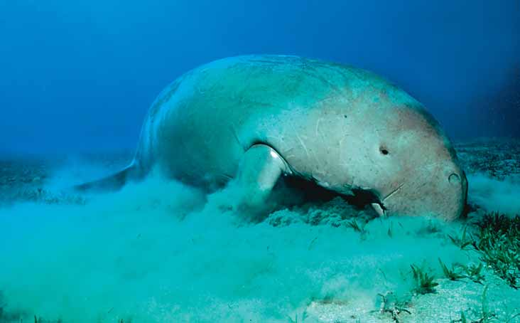
9
MARINE MAMMALS
9.1 INTRODUCTION
The marine mammal fauna of the Red Sea and Gulf of Aden
is not well known. Although 44 species of cetacean (dolphins,
porpoises and whales) and one species of sea cow (the dugong)
are known from the Indian Ocean, only 15 species have been
reported from the Gulf of Aden and 11 from the Red Sea
(Table 9.1). However, the species list for the Red Sea is known
to be incomplete. No baleen whales have been reported for the
Red Sea, yet three whales (suspected of being Bryde's) were
seen on each of two aerial surveys of the Farasan Islands area (in
August 1987 and September 1993; PREEN unpublished data).
The fact that these whales appear to be common in the southern
Red Sea, but have never been reported, demonstrates the need
for more survey work.
Of the 16 species of marine mammal confirmed from this
region, three are listed as threatened species (endangered or
vulnerable), five are considered dependent upon specific
conservation efforts to prevent threatened listing, five are
insufficiently known to ascribe any status and three are
considered secure (IUCN 1996; Table 9.1). These figures
highlight the need for more information on the marine mammals
of this region. Only with data on distribution, abundance and
267

---

Standard Survey Methods
threats can effective management be
protect threatened populations of dugongs
implemented for the conservation of this
(e.g. eastern Australia; DPI 1998; PREEN &
important group of animals.
MORISSETTE 1997) and some small cetaceans
(e.g. Banks Peninsula, New Zealand, DAWSON
& SLOOTEN 1993; upper Gulf of California,
Worldwide, cetaceans and dugongs face
Mexico, REEVES & LEATHERWOOD 1994).
many threats. While the large whales still
Marine pollution by oil or other chemicals is
suffer from legal and illegal whaling
an ever-present threat. Although the evidence
operations, a more insidious and widespread
for a link between chemical pollution and the
threat is posed by mesh nets, which are
health of marine mammal populations remains
predominately used to catch fish. In recent
largely circumstantial, there is growing
decades the proliferation of synthetic gill nets
concern that large contaminant loads can
throughout the world has posed a serious
increase susceptibility to disease and affect
threat to some cetaceans, dugongs, seabirds,
reproduction. Disturbances from shipping,
turtles and fish. In 1990, six stocks of
military activities (e.g. target practice, depth-
cetaceans were identified as suffering
charge practice), seismic exploration for oil,
unsustainable mortality in net fisheries
and increased boating activity have also been
(COOKE 1991). Sanctuary areas, where mesh-
identified as potential threats to marine
nets are banned, have been established to
mammals (COOKE 1991; FRAZIER et al. 1987).

IUCN
Distribution
Rarity
Species
status
& Reference 1=more common
2=less common


GA
RS

Dugong
Dugong dugon VU
1
5
1
Blue whale
Balaenoptera musculus EN
2,4
2
Bryde's whale
Balaenoptera edeni DD
2

1
Sperm whale
Physeter macrocephalus VU
2,4
1
Melon-headed whale
Peponocephala electra
2

2
False killer whale
Pseudorca crassidens
2
3,4
2
Killer whale
Orcinus orca CD
2
4
2
Short-finned pilot whale
Globicephala macrorhynchus CD 2,4
1
Indo-Pacific humpbacked
Sousa chinensis DD
2
3,4
1
dolphin
Common dolphin
Delphinus delphis
2
4
1
Bottlenose dolphin
Tursiops truncatus DD
2
3,4
1
Risso's dolphin
Grampus griseus DD
2
3,4
1
Pantropical spotted dolphin
Stenella attenuata CD
2
3,4
1
Striped dolphin
Stenella coeruleoalba CD
2
4
2
Spinner dolphin
Stenella longirostris CD
2
4
1
Rough-toothed dolphin
Steno bredanensis DD

4
2
1. ROBINEAU & ROSE 1982. 2. SMALL & SMALL 1991. 3. BEARDON 1991. 4. FRAZIER et al. 1987. 5. PREEN 1989.
Table 9.1 Species of marine mammal reported from the Red Sea (RS) and Gulf of Aden (GA), and their
conservation status. IUCN (1996) categories: EN: endangered; VU: vulnerable; CD: conservation dependent;
DD: data deficient.
268

---

Marine Mammals
There is little specific information about
in properly surveying marine mammals, it is
threats facing marine mammals in the Red Sea
important to clarify the objectives of the
and Gulf of Aden. Perhaps most is known
survey, to reconcile these with the resources
about the dugongs, at least along the eastern
available and to select the most appropriate
coast of the Red Sea (Saudi Arabia and
method.
Yemen). In 1987, the dugongs in this area
were censused by large scale aerial surveys,
and fishermen were interviewed to learn about
9.1.2 Survey objectives
threats to the dugongs (PREEN 1989). That
study estimated there was a population of
In a region like the Red Sea and Gulf of
2000 dugongs in the eastern Red Sea and that
Aden, where there is relatively little existing
the level of fish-net related mortality of
information, the objectives of any surveys
dugongs was low in most areas. The one area
should reflect the information needs.
where net mortality levels may have been
unsustainable (the Gizan and Farasan Islands
area) was resurveyed in 1993 and the results
The most basic needs for informed
suggested a decline in dugong numbers
management are:
(PREEN unpublished data). Very little is
known about the dugong populations along
A list of the species present
the western shore of the Red Sea or in the Gulf
of Aden. Even less is known about most
The broad distribution of each species
species of cetacean. There is a genuine need
for marine mammal surveys to be conducted
Some measure of the abundance of
in this region before it will be possible to
each species
make confident statements about the status of
The particular habitat requirements of
any species.
each species, and
The main causes of mortality or threats
9.1.1 Surveying marine mammals
to the marine mammals in the region.
Marine mammals are highly mobile and
Measurement of abundance can be
move over very large areas. Even species
difficult. Two measures are used: absolute
thought to be relatively sedentary, such as
abundance and relative abundance. The
dugongs, can be highly mobile. Satellite-
absolute or actual abundance can be very
tracked dugongs have moved between areas
expensive to determine accurately. Relative
up to 700 km apart over a two-week period
abundance, by contrast, is an index that
(PREEN 2000). Furthermore, marine mammals
reflects actual abundance. Many survey
are rare compared with most marine life.
methods that have the potential to measure
Consequently, surveys of marine mammals
absolute abundance really measure relative
must cover large areas and must expect only a
abundance. This occurs when accurate
low rate of encounter. The need to cover large
detection functions and correction factors,
areas often means that surveys are expensive
which are necessary to correct for animals that
to conduct. The low sighting rate has
are deep below the surface and are
implications for the accuracy and precision of
undetectable, have not been derived. This is
population estimates derived from the surveys
generally not a problem as good measures of
and a comparatively high coefficient of
relative abundance are adequate for most
variation of the result can generally be
purposes. Good data on relative abundance
expected. Because of the difficulties involved
will allow the monitoring of the size of a
269

---

Standard Survey Methods
population through time (as long as the
9.1.3 Selection of methods
repeated surveys exactly duplicate the
previous surveys).
There are many survey methods, ranging
from the simple to the highly sophisticated,
from the inexpensive to the very expensive.
9.1.2 Available resources
Table 9.2 provides an incomplete list of
methods with an indication of the type of
The realistic objectives of a survey and the
information they can provide and the
selection of the most appropriate survey
resources they require. It is important to
method will be dictated largely by the skills
realise that there is no single best technique
and training of the researchers, the facilities
(ARAGONES et al. 1997). Different methods
available and the size of the budget.
will be appropriate to different surveys,
Generally, the methods that provide the most
depending on their objectives and the
quantitative data are sophisticated and
resources that are available.
expensive to implement properly.
Furthermore, they require substantial logistic
support and high levels of training.





Method
Information provided
Spatial
Technical
Cost
scale
requirements





Interview
Distribution, relative abundance,
large area
low
low
survey
habitat preferences, most important
areas, mortality factors, population
trends





Carcass
Species list, unusual causes of
limited
low to high
low to
salvage
mortality, seasonality of mortality,
area
high
aspects of biology (age, diet,
reproductive history, genetics)





Transect
Species list, distribution, relative
medium
medium
medium
boat
abundance, absolute abundance (with
area
surveys
adequate correction factors),
monitoring abundance through time,
human activities in the study area





Shoreline
`Hot spot' areas for coastal marine
large area
low
medium
aerial
mammals, distribution of species,
surveys
distribution of habitats, human activities
in the study area





Transect
Distribution, relative abundance,
large areas high
high
aerial
absolute abundance (with adequate
surveys
correction factors), monitoring
abundance through time, use of
different habitats, extent of preferred
habitats
Table 9.2 Summary of the attributes of the main survey methods for marine mammals.
270

---

Marine Mammals
9.2 METHODOLOGY
Expertise needed
Some knowledge of interview techniques
and questionnaire design is required. Good
9.2.1 Interview Surveys
interpersonal skills and fluency in the local
language, or the aid of a good translator, is
Introduction
essential. Knowledge of the people to be
Interview surveys are a useful and
interviewed and their culture is important. The
inexpensive first step in establishing a
interviewer must also have a good knowledge
database of marine mammals for a region.
of the marine mammals that may occur in the
Fishermen, and other knowledgeable people,
area.
can be interviewed to learn from their
experiences with the various species present
in the region. When working in an area where
Equipment needed
little information exists, interview surveys can
A vehicle would be required to move from
provide the most information for the least
settlement to settlement along the coast. A
expense. Interview surveys can identify
collection of laminated photographs of the
particularly important areas for marine
animals expected in the area (and some that
mammals. They may also be used to evaluate
could not be in the region) is very useful.
the conservation interest of local people and
for initial education. Subsequent repeat
surveys can assess the impact of education or
Costs
conservation projects. Interview surveys are
There are few expenses other than salaries
most useful for inshore species, such as
and the cost of transport.
dugongs and some species of dolphin, with
which people are most likely to interact.
Because they are inexpensive to implement,
Method
interviews can be conducted along extensive
Interviews can be formal or informal. An
sections of coastline, thus providing regional
informal, semi-structured approach, where the
data.
interview can take place as a directed
conversation is often most successful when
there are only a few knowledgeable people.
Information that can be obtained
This approach may also be best if the
Interview surveys can provide information
interviewers may be perceived as
on the distribution of species and subjective
representatives of the government, and a level
data on their relative abundance. They may
of suspicion and intimidation has to be
also provide subjective views of trends in
overcome. Good rapport must be established
abundance over years to decades. Interview
before the interview is conducted. This may
surveys can provide information on the
take some time. Interviews cannot be rushed
sources and levels of mortality, on hunting
and must develop and proceed at a rate that
and capture methods, and on uses made of the
the informant is comfortable with. Some
animals. Information on habitat preferences,
fishermen are particularly observant and
aspects of biology (such as movement
knowledgeable. When such fishermen are
patterns, breeding season, and food) may also
encountered it may be desirable to extend the
be provided. Awareness of conservation
relationship with the informant(s) over several
efforts and relevant laws may also be
visits.
evaluated.
271

---

Standard Survey Methods
Following initial formalities and the
In areas where there is a high level of
development of trust, interviews should
human activity in the coastal waters, such as
usually start with a series of descriptive
around coastal cites, sighting sheets can be
questions, where the informant is encouraged
used to collect information about marine
to describe what he has observed or learned.
mammals. An example of a sheet that could be
These questions can lead to more structured
adapted for use in the region is included in
questions, where the informant is asked to
Appendix 9.6.2. Such sheets can be
provide detailed information about particular
distributed to people who regularly spend
areas of interest and knowledge. The
time in boats in the area of interest. The
interview must also include a range of
information provided is often of limited use
contrast questions. These aim to check the
due to the unreliability of the identifications,
reliability of the informant, and therefore the
and the non-random sampling effort.
validity of the information he is providing.
However, when used with other survey
Contrast questions may include queries to
methods which may verify the data provided,
which the answers are already known, as well
sighting sheets can provide useful
as questions to which the informant could not
supplementary information on distribution
possibly know the answer (e.g. life history
and group sizes. Moreover, such sighting
data that can only be derived by scientific
sheets are very useful in increasing public
techniques).
awareness of marine mammals.
It can be very helpful to have photographs
A set of outline drawings of the marine
of the different marine mammals that may
mammals listed in Table 9.1, together with a
occur in the area. It should be noted that the
sketch of their skulls, is provided in Appendix
identification of some dolphins is very
9.6.3. These may prove useful for the
difficult and some identifications made by
identification of live or dead specimens.
informants may not be accurate. Inclusion of
Readily available guides to the identification
photos of some distinctive species that do not
of cetaceans include JEFFERSON et al. (1993)
occur in the region can be useful for assessing
and LEATHERWOOD & REEVES (1983).
the reliability of species identifications. Skull
bones (or photographs of them) can also be
helpful in stimulating conversation and
9.2.2 Carcass Salvage
establishing rapport. It is common for there to
be skull bones of whales, dugongs or dolphins
in fishing villages. These should be
Introduction
photographed and identified where possible.
Marine mammals that wash up on beaches
can be a useful source of information. Beaches
can be driven or walked in search of beached
Appendix 9.6.1 lists the type of
carcasses or old skeletal material. In more
information sought from fishermen in Saudi
populated areas local people can be encouraged
Arabia and Yemen to help assess status of
to report carcasses. A carcass salvage
dugongs along the eastern Red Sea (PREEN
programme can be simple and inexpensive or
1989). That study also included detailed aerial
sophisticated and expensive, depending on its
surveys to estimate the numbers of dugongs in
aims and the facilities and expertise available.
the region. Consequently, the interviews
Carcass salvage is often unpleasant work as the
focussed on the numbers of dugongs killed in
animal has often been dead for a period of time.
nets or by hunting.
Despite the unpleasantness, carcass salvage is
important work.
272

---

Marine Mammals
Information that can be obtained
maps and a GPS to record the location of
At the most basic level, carcasses of
specimens should be used. A necropsy kit
marine mammals provide evidence for the
should contain a range of surgical gear from
presence of the species in the region. Although
large knives to scalpels, plastic bags,
species identification may be easiest with
containers and labels for samples, a
recently dead carcasses, old skulls found high
measuring tape, a camera, gloves and clean-
on the beach can also be identified and DNA
up materials. Caution should be taken not to
can be extracted from dried skin (and perhaps
cut yourself, especially when dealing with
even old bones) to determine identification.
rotting carcasses. The necropsy kit should
Carcasses of marine mammals can also
include appropriate data sheets and a simple
provide information on the causes and rates of
guide to the identification of marine mammals
mortality of species (e.g. if they are dying in
in the region (Appendix 9.6.4).
nets the carcasses sometimes retain
characteristic marks). Repeated surveys of
long stretches of coast conducted at yearly
Costs
intervals may provide information on the
Implemented at its basic level, carcass
normal rate of mortality in the region, and thus
salvage is inexpensive as the main costs are
may highlight any unusual increases. Surveys
salaries and transportation. Analysis of tissue
repeated more frequently over smaller
samples can be expensive.
sections of coast can identify any seasonal
patterns in mortality (sometimes such peaks in
beached carcasses relate to certain types of
Method
seasonal fishing activity). If facilities and
The fresher the carcass the more
training are available, freshly dead carcasses
information can be collected. An extremely
can provide samples that can be analysed to
fresh carcass (hours old, depending on
provide information on the biology of the
ambient temperature) can provide samples
species (e.g. age, age of sexual maturity,
and data that give information on
fecundity, season of mating and birthing, diet,
bacteriology, virology, haematology and
genetics). Tissues can also be analysed for
pathology. However, there is little need for
levels of pollutants, parasites and pathogens.
such information until a great deal is already
known about the populations of marine
mammals in the region and the threats they
Expertise needed
face. Moreover, the skills required and the
The ability to identify the marine mammal
expense involved for the collection, analysis
species of the area and knowledge of their
and interpretation of this type of information
basic anatomy is required. Experience of
are considerable.
necropsy procedures and techniques for the
proper collection and preservation of specific
tissue samples is also highly desirable. Such
A carcass that is hours to days old may
samples can be sent to specialists for analysis
provide information on parasites,
if local facilities and expertise are
contaminants (by analysis of tissue samples),
unavailable.
cause of death (from marks on the body), diet
(by analysis of stomach contents), age (by
analysis of growth layers in the teeth), gender,
Equipment needed
reproductive stage (by examination of gonads
A
four-wheel drive vehicle with
and reproductive tract) and genetics (by
appropriate safety and self-rescue gear is
analysis of skin or gonad samples). Some of
required for travel along beaches. Suitable
these analyses require special expertise or
273

---

Standard Survey Methods
experience. However, most of the samples can
9.2.3 Line-Transect Boat Surveys
be collected and preserved by someone with a
good knowledge of the anatomy of cetaceans
Introduction
and dugongs, and basic necropsy training.
A boat with an elevated viewing platform
follows a predetermined path and observers
search each side and in front of the boat for
Even a rotten carcass that has been dead
marine mammals. Once sighted, the distance
for days to weeks can provide data on species
to each group and the angle of each group
present (identification based on measurements
from the transect is recorded, along with
of the extracted and cleaned skull), age, body
information about the number and species of
length and genetics. Sometimes it is still
marine mammals in the group.
possible to determine the gender of the
animal, and in the case of dugongs the
stomach contents may still be intact. As the
Information that can be obtained
carcass ages further only the skull and perhaps
Boat surveys can provide quantitative
a piece of dried skin can be collected. Even
information on the abundance and distribution
these samples can allow the carcass to be
of cetaceans at the species level over large
identified to species, aged, and its genetic data
areas. When repeated regularly in an area,
to be determined.
these surveys can identify seasonal
distribution and movement patterns. Repeated
surveys can also be used to monitor changes
GERACI & LOUNSBURY (1993) provide a
in the abundance of species over time.
detailed guide to the anatomy and sampling of
Because a lot of time is spent on the water,
marine mammal carcasses. A detailed manual
this method can provide insights into
for the necropsy of dugongs can be
conservation issues in the area. Boat surveys
downloaded from <www.gbrmpa.
are not effective for surveying dugongs as this
gov.au/corp_site/info_services/publications/
species spends very little time near the
research_publications/rp64/index.html>.
surface. Boat surveys are effective for
Much of the information in this manual is
surveying large cetaceans only if the whales
applicable to cetaceans. Appendix 9.6.4
are very common in the region, or the surveys
includes a simple identification guide and a
cover very large areas extending long
data sheet for recording basic information
distances from the coast. Generally, such
from a carcass in English or Arabic (PREEN et
surveys require large ocean-going vessels, and
al. 1989). Appendix 9.6.5 contains a detailed
are very expensive to conduct.
data sheet for the recording of full
morphometric data from cetacean carcasses.
Appendix 9.6.6 is a data sheet specifically for
Expertise needed
dugongs that can help guide the necropsy and
This method requires trained observers
be a reminder of the samples to collect.
that can identify cetaceans confidently. The
Ideally samples and data should be lodged
design of surveys and the analysis of the data
with national museums where they can be
requires a high level of training, including
professionally stored and kept for future
knowledge of line transect methodology,
reference and study.
statistical skills and access to appropriate
software.
274

---

Marine Mammals
Equipment needed
Marine mammals can be difficult to
A suitable vessel is required with a depth
identify, so the spotting team must include at
sounder, GPS (often present as part of the
least some trained observers. A minimal
vessel's navigation equipment), binoculars,
survey team would consist of two trained
sighting compass, data sheets, charts,
observers. One observer would continuously
computer and software.
search the path in front of the boat (from 9
o'clock to 3 o'clock if the boat is assumed to
be pointing to 12 on a clock face) with
Costs
binoculars (7 x or 8 x). The other observer
Boat time can be expensive, although it is
would search for animals directly on the boat
possible to conduct these surveys on small
path with the naked eye (to assure optimal
local craft if a suitable platform can be erected
compliance with assumption 1, below), and
and the seas are calm. The associated
acts as data recorder for the primary observer.
equipment can also be expensive. Several
A larger team would have four observation
observers are required to search either side of
positions, a data recorder, and a rest station.
the boat thoroughly and allow for rest periods
Position 1 would search the transect in front
to reduce fatigue.
of the boat from 9 o'clock to 3 o'clock using
powerful binoculars (up to 20 x) that may be
mounted on the deck. Positions 2 and 3 would
Method
be located on each side of the viewing
The survey should be designed to cover
platform and search 9 o'clock to 12 o'clock
the entire survey area and the transect lines
and 3 o'clock to 12 o'clock, respectively, using
should be random with respect to marine
7 x or 8 x binoculars. The observer in position
mammal distribution. If a relatively small
4 would search the transect directly in front of
boat is used it may be necessary to design the
the boat with the naked eye.
transects to allow the boat to be in a port each
night. The density of the survey lines will
depend on the size of the area to be surveyed.
When a sighting is made, the boat may be
Detailed surveys of relatively small areas,
stopped and the following information
which seek to determine fine-scale
recorded:
distribution, may have transects as close as
1 km apart (e.g. JEFFERSON & LEATHERWOOD
Time, position (from GPS)
1997). In regional surveys, covering
thousands of square kilometres, transects may
Sighting angle (the angle between the
be 5­20 km apart (e.g. DOLAR et al. 1997).
compass bearing to the group and the
compass bearing of the transect)
The size of the boat used for a line transect
Sighting distance
survey will depend on the extent to which the
Group size
survey covers offshore waters, where
conditions may become rough. Higher
Associated animals
observation platforms are more likely on
larger boats. Observers should be at least 3 m
Notes on interesting behaviours and
above water level. Boat speed while on-
Basic oceanographic data (e.g. water
transect should be about 7­8 knots (kn)
temperature, salinity and depth).
(13­15 km/h).
275

---

Standard Survey Methods
The sighting data should be recorded in a
All groups actually on the transect are
standardized format (see Appendix 9.6.7). A
detected. This is unlikely to be met
GPS can provide vessel path and speed.
with cetaceans and dugongs and will
Periodically (e.g. every 15 min.) sighting
result in negative bias in abundance
conditions (Beaufort sea state, visibility)
estimates. Detection functions have
should also be recorded. Sighting distance
been developed for some species to
may be estimated by eye after training. It may
correct for missed groups (BUCKLAND
be checked by taking a GPS point from the
et al. 1993) and some surveys have
position in which the animals were first seen
towed cetacean detectors behind the
and comparing this to the boat's position at the
boat to determine the proportion of
time of the initial sighting. Sighting angles
some species that are missed by the
can be measured with binoculars with an
observers (JEFFERSON 2000). In most
inbuilt compass or a good sighting compass
situations, however, it is a matter of
could be used. Observations should only be
diligent observation to ensure minimal
made under relatively good conditions, that is,
violation of this assumption.
Beaufort sea state 4 (Table 9.3).
Animals are observed and recorded
before they move in response to the
Data analysis
boat.
Line-transect methods use the information
Sightings are independent of each
on the distribution of perpendicular sighting
other.
distances and the amount of survey effort to
estimate density and abundance. This
The average group size for each
methodology requires that a series of
species is estimated without bias.
assumptions are met if unbiased abundance
estimates are to be obtained (B
Sighting angles and distances are
URNHAM et al.
1980). The main assumptions are:
measured accurately.





Beaufort
Description of wind
Sea conditions
Wind
Wave
value
speed
height
(knots)
(cm)





0
Calm
Smooth, mirror-like
0-1
0





1
Light air
Scale-like ripples
1-3
7





2
Light breeze
Small short waves, crests have glassy
4-6
15
appearance and do not break





3
Gentle breeze
Large wavelets; some crests begin to
7-10
60
break; foam of glassy appearance;
occasional white foam crests





4
Moderate breeze
Small waves, becoming longer;
11-16
120
frequent white foam crests (`white
horses')





5
Fresh breeze
Moderate waves taking a more
17-21
200
pronounced long form; many `white
horses', there may be some spray
Table 9.3 Abbreviated Beaufort scale for ranking sea state and estimating wind speed.
276

---

Marine Mammals
Perpendicular sighting distance is
estimates of density and abundance. It is
calculated from the sighting distance and
recommended (BUCKLAND et al. 1993) that the
sighting angle using the formula:
perpendicular distance is truncated at a certain
distance to remove outliers, improve the
modelling and reduce the coefficients of
y =r sin
variation. Typically only the most distant
where
2­3% of sightings are removed.
y = perpendicular sighting distance
r = sighting distance
9.2.4 Shoreline Aerial Surveys
= sighting angle
Introduction
Density and abundance, and their
This is a relatively simple and inexpensive
associated coefficients of variation are
method of identifying some of the most
estimated using the following formulae:
important habitats for inshore species,
particularly dugongs. A light aircraft is flown
at low altitude over near-shore waters and the
D = [n f (0) E(s)] / 2L
location and number of marine mammal
groups, and the habitat in which they are seen
N = [n f (0) E(s) A] / 2L
is recorded onto maps. The flight path usually
searches areas that are expected (on the basis
CV = {[var (n) / n2] + [var ( f (0)) / ( f (0))2]
of information from interview surveys or
+ [var (E(s)) / (E(s))2]}
other sources) to be suitable for dugongs or
where:
inshore cetaceans.
D = individual density
Information that can be obtained
n = number of sightings
This method can identify 'hot spot' areas
f(0) = value of the probability density
where marine mammals are common and can
function
give the researchers a good appreciation of the
distribution of habitat types in the region.
E(s) = mean group size
Information on the distribution of turtles,
seabirds and human activities (e.g. fishing,
L = length of transect surveyed
location of villages, location of coastal
N = individual abundance
developments, etc.) can be collected at the
same time. Frequently repeated surveys may
A = size of the study area
provide information on the seasonality of
occurrence of species in a region. However
CV = coefficient of variation
such data should be treated cautiously and as
var = variance
preliminary, as such a very small proportion
of the sea surface in an area is actually
The calculation of f (0) requires
searched during shoreline surveys
complicated mathematics and statistics. A
(consequently, the absence of evidence is not
computer programme called DISTANCE (LAAKE
necessarily the evidence of absence).
et al. 1994) is available to derive f (0) and the
277

---

Standard Survey Methods
Expertise needed
Fuel availability can be an important
The identification of marine mammals
logistical constraint in some areas. It may be
from the air can be difficult and considerable
necessary to arrange fuel dumps beforehand
experience is required to get reliable
for effective coverage without losing
identifications. Basic cartographic skills are
excessive amounts of flying time to refuel. In
required for designing the flight path and the
some areas (e.g. Arabian Peninsula) the
accurate plotting of sightings.
availability of fixed-wing aircraft fuel (Avgas)
is very limited and it may be necessary to use
helicopters (Jet A1 fuel is more widely
Equipment needed
available). Sometimes it is possible to get
Maps and binoculars are essential. To
support from military aircraft for surveys.
reduce the effects of aircraft vibration,
binoculars should not be too strong (8 x) and
should have a large-diameter lens near the
9.2.5 Transect Aerial Surveys
eye. A camera is highly desirable. A GPS can
be helpful, but is not essential as it is usually
possible to navigate accurately from coastal
Introduction
features.
A suitable aircraft is flown along
predetermined parallel flight lines (transects)
and the location of sightings is recorded. With
Costs
strip-transect aerial surveys the aircraft
The charter of the aircraft and pilot is the
usually has a frame or other device on the
main expense. However, large areas can be
outside of the aircraft to demarcate the
covered in a relatively short period, usually
predetermined width of the search area. Only
making this method cost-effective.
sightings within this area are included. A high
level of rigour is required in the flying of the
aircraft (maintaining exact altitude and flight
Method
line) and in the recording of the sightings if
A helicopter or high-wing aeroplane (for
repeat surveys are to be compared. The
an unimpeded view of water) can be used; the
method is most suited to surveys of large
former is more expensive to operate. A
areas, where the water is relatively clear. It is
single-engined aircraft is suitable as the
generally limited to near-shore waters (up to
aircraft is rarely far from land. The aircraft is
about 60 km from shore) due to refuelling
typically flown at an altitude of about 700 ft
logistics.
(400­900 ft; 122­274 m) at a ground speed of
90­100 kn (167­185 km/h). Good survey
conditions are required for high sighting
Information that can be obtained
rates: low cloud cover, surface wind 15 kn
This is a reliable method of estimating the
(28 km/h; Beaufort sea state 3). Water
abundance and distribution of many species
clarity can vary with season (depending on
over large areas. With appropriate correction
direction and strength of wind as well as
factors it is possible to derive estimates of
rainfall/run-off events) and surveys are best
absolute abundance. The use of different
conducted when the water is clearest.
habitats and the extent of preferred habitat can
Observers should wear polarized sunglasses
be determined. The same surveys can be
to minimise the effects of reflected glare.
repeated at intervals of several years to
monitor changes in the size of populations
(e.g. PREEN in press). The same surveys can
also be repeated at much shorter intervals to
278

---

Marine Mammals
eye
b'
Wing Strut
a'
b
Window
a
h
A
B
Figure 9.1 Calibrating transect markers
1.
Prop the aircraft into the flying attitude.
2.
Sit first observer in their seat and get them to 'sag' into a comfortable and realistic position for observing.
3.
Measure the height h, that is, the height of the observer's eye above the floor.
4.
Fix the position of the inner transect marker (a) so that it is close to the aircraft body, without being obstructed by
the bottom of the window.
5.
Put a mark, A, on the ground, and a mark a' on the window such that the observer's line of sight passes from a'
through a to A.
6.
Place a second marker on the ground at B. The distance between A and B is derived from the formula:
w = W . h/H where:
W = the required transect width (e.g. 200 m or 215 m)
H = the flying height
7.
While the observer maintains the a' ­ A line of sight, he puts a second mark on the window at b'.
8.
The outer transect marker is adjusted to position b, such that the observer has a straight line of sight b' through
b to B.
9.
Repeat for the observer on the other side of the aircraft.
If two observers are used on each side of the aircraft then the position of the transect markers is defined by the mid-seat
observers. The rear-seat observers must mark their windows with a' and b' marks so that they are observing the same transect
as the mid-seat observers. They may need to use cushions to adjust their head height.
If the observers always keep their heads in the correct observation position then the transect width defined by the lines a'­a
and b'­b will define the correct transect width, when flying at the correct altitude (Figures 9.1 and 9.2).
determine the seasonal distribution of species,
Expertise needed
which is important information for
A crew of at least two observers, plus a
management planning. Such information may
flight controller is required as well as the
also provide insights into movement patterns
pilot. The observers need to be experienced at
and ecological links with neighbouring
identifying marine mammals from the air and
countries. Transect aerial surveys can also
must not be prone to motion-sickness. The
provide very valuable data on the distribution,
design and analysis of transect aerial surveys
habitat use and abundance of marine turtles
requires the controller to have a sound
and seabirds, as well as data on fishing and
understanding of strip- and line-transect
other vessels, nets and fish traps, and oil
methodology and good statistical, computer
pollution incidents.
and cartographic skills.
279

---

Standard Survey Methods
Equipment needed
expensive, but once purchased or assembled is
High-wing aircraft with a very low
available for subsequent surveys. The salaries
stalling speed or helicopters are suitable for
of the observers and the time-consuming
this work. Helicopters are usually much more
analyses must also be accounted for.
expensive to charter (unless military
assistance is available) and tend to have lower
endurance. For safety reasons a twin-engined
Method
aeroplane is desirable if the transects extend
Strip-transects are a special type of line-
far out to sea. Ideally the aircraft will have a
transect where it is assumed that all animals
GPS and a radar altimeter. Observers require
visible within the width of the transect are
polarized sunglasses. The controller requires
seen. To ensure that this occurs, the transect
binoculars, maps, data sheets or computer. An
width is very narrow. On dugong surveys it is
intercom for communication between the
usually 200 m on each side of the aircraft.
observers and the controller is virtually
essential. A computer is necessary for data
analysis. A tape recorder is useful for
The advantage of the strip-transect survey
documenting observations and is essential if a
is that it is not necessary to measure the
larger team of observers is used.
distance and angle to each sighting, as
required for line transects. This is important in
near-shore environments where many animals
Costs
(dugongs, turtles, dolphins, seabirds) and
This type of survey is expensive to conduct
human activities (fishing boats etc.) may be
due to the large number of flying hours
seen in close proximity1.
involved. Ancillary equipment can be
Line of Sight from b' to b
Line of Sight along
Lower Window Edge
a' to a
152 m
Sea Surface
200 m
200 m
Figure 9.2 Plane flying with transect widths of 200 m
1 Line­transect surveys are more frequently used for open ocean surveys of cetaceans, where the sighting rate is much lower.
If open­ocean species of cetacean are the taxa of interest then it is necessary to modify the line transect boat surveys, described
above, for aircraft.
280

---

Marine Mammals
Strip-transect aerial surveys are typically
Any change in flying height affects the
designed to cover large areas
effective transect width and, hence, the
(5,000­50,000 km2). Transect density will be
sampling intensity (Figure 9.2). The altitude
determined, in part, by the amount of suitable
of the aircraft must be kept constant during
habitat in the survey area: transects should be
surveys and, if using a barometric altimeter,
denser in areas where animals are more likely
deviations as a result of air pressure changes
to be encountered. For the estimation of
during the flight must be measured. This is
regional densities, the survey area is usually
done by recording the difference between the
stratified into blocks, and these may have
actual elevation of the airstrip where the
different transect densities. Typically transects
aircraft lands with the altitude of the strip
are about 9­10 km apart in areas of probable
measured with the barometric altimeter.
low density (such as offshore areas) and
3­4 km apart in areas of better habitat.
Tighter transects may be flown in smaller
The 'sightability' (the ability to spot and
areas where the major aim is to produce a
identify) of smaller marine mammals and
detailed plot of distribution.
turtles declines as survey conditions
deteriorate. If surveys are to be repeated to
monitor populations over time, it is essential
Flight efficiency (or cost) usually dictates
that survey conditions are kept as similar as
that transects are arranged parallel to each
possible for each survey. Surveys should be
other. Therefore, at least the position of the
conducted in the season of lowest winds (based
starting transect should be selected randomly.
on meteorological data where possible, or on
Ideally, transects should run perpendicular to
the knowledge of experienced fishermen).
the depth contours.
During surveys, flying should only be
conducted when the wind is less than about
15 kn (28 km/h; Beaufort sea state 3). To
Transect markers may take the form of a
reduce the effects of reflected glare, surveying
frame or fixed rods attached to the wing struts
should not be conducted during early mornings
and wheel supports of the aircraft (see
or late afternoons. Unless the sea is very calm,
Figure 9.1). A simpler method involves using
glare is usually unacceptable during the middle
a thin rope trailing from the wing struts. A
of the day as well. Observers should wear
funnel attached to the free end of the rope
polarized sunglasses to reduce the effects of
ensures that the rope flies straight and
glare.
horizontal. Attaching transect markers to
helicopters is more difficult due to the safety
issues related to detached markers getting
The survey team will consist of a controller
caught in the rotor blades. Approval for any
and either two or four observers, depending on
external attachments may have to be obtained
the configuration of the aircraft. Four observers
from the aviation authorities. Figure 9.1
are desirable, as more precise perception bias
shows how to adjust the transect markers to
correction factors can be derived.
achieve the desired transect width.
If only two observers are used (one on each
The aircraft flies at an altitude of 500 ft
side) the controller must act as a part-time
(152 m) and a speed of 90­100 kn
observer and periodically rotate the sides of the
(167­185 km/h) while on the transect.
observers. When four observers are used, two
search the same area on each side of the
aircraft. The two observers on each side must
281

---

Standard Survey Methods
be visually and acoustically isolated from each
then the altimeter height of the airstrip is
other so their observations are independent
recorded at each take off and landing. This
(one cannot take a cue from the comments or
information, with the actual airstrip altitude, is
behaviour of the other). Curtains are used for
used to correct the altimeter measurements of
visual separation while the intercom ensures
flying height for each transect.
acoustic isolation.
For aerial surveys to be used to estimate
A four-observer team requires an aircraft
abundance and to monitor trends in abundance
with six seats that provide clear views of the
through time, it is necessary to correct for the
search area. The pilot and controller sit in the
number of animals not seen by observers.
front seats, with two observers (port and
Following MARSH & SINCLAIR (1989)
starboard) in each of the mid and rear seats.
corrections are needed for two types of bias:
While on transect the mid-seat observers can
talk to one another and to the controller, while
1. Perception bias: those animals that are
the rear-seat observers can only communicate
visible within the transect, but are
with each other. Between transects and during
missed by the observers. Correction
transit the intercom is opened up for free
factors are calculated by using paired
communication. All communications are
but independent observers, one behind
recorded by a stereo tape recorder for later
the other. The numbers of animals
transcription. These tapes make it possible to
seen or missed by each observer are
determine the degree of agreement between
used in a mark-recapture analysis to
paired observers so the perception bias
estimate the proportion of animals
correction factors can be derived. During the
missed by either or both observers.
survey the controller records the sightings of
the mid-seat observers onto a computer or onto
2. Availability bias: those animals that
data sheets. These data act as a backup in case
are below the surface and are not
of tape failure. Appendix 9.6.8 provides data
visible. A correction factor for this bias
sheets for strip transect aerial surveys.
is estimated by
a) recording during the survey which
The following information is recorded for
animals are at the surface and
each observation: time, transect, direction the
b) studying individuals of the same
transect is flown, observer, number in group,
species to determine what
number at surface, number of calves, position
proportion of time they spend at
in transect, species and confidence of species
the surface.
identification. Position in transect (high,
middle, low) is used to distinguish between
The extent to which surface time
simultaneous sightings made by observers on
varies between place, time, water
the same side of the aircraft. The start and end
depth and behaviour is not known, but
times of each transect are also recorded and
is likely to reduce the accuracy of
the location of each sighting is based on
availability bias correction factors.
elapsed time and the known length of each
However, as better data become
transect. Information on sighting conditions
available, correction factors can be
(Beaufort sea state and level of glare on each
adjusted and previous surveys re-
side of the aircraft) and flying height is
analysed.
recorded every few minutes. If a barometric
altimeter is used to maintain survey height
282

---

Marine Mammals
9.3 DATA ANALYSIS
ACF = availability correction factor
After the survey the tape records of each
CV = coefficient of variation of the
transect are used to edit the controller's record
estimate of the ACF
of the sightings of the mid-seat observers.
ps = the proportion of animals seen at the
Each sighting is identified as made by the mid-
surface during an aerial survey of clear-
seat, rear, or both observers on the relevant
water habitat where all animals could be
side. The perception bias correction factors for
seen
each pair of observers and its coefficient of
variation are estimated using the following
pu = the proportion of animals seen at the
formulae (MARSH & SINCLAIR 1989):
surface during the aerial survey being
analysed
PCF = [(S
N
m + b)(Sr + b)] / [b(Sm + Sr + b)]
u = the total number of animals (e.g.
dugongs) seen during the aerial survey
and
Ns = number of animals (e.g. dugongs)
seen during a survey of clear water habitat
CV = [(Sm + Sr) / (Sm + Sr + b)] * {(Sm*Sr) /
[b(Sm + b)(Sr+ b)]}
An estimate of ps may be derived by other
methods, including multiple records of
where:
surfacing and diving intervals of a large
number of individuals or the use of time-depth
recorders. Differences in habitat, water depth
PCF = perception bias correction factor
or behaviour may mean that the proportion of
CV = coefficient of variation of the
animals at the surface may not be the same for
correction factor
the two sets of data used to derive ps and pu.
However, the ratio of pu/ps provides a useful
Sm = number of groups seen by the
means of standardizing fluctuating
mid-seat observer only
availability bias for repeat surveys of the same
area. The ratio 80:480 has been used as an
Sr = number of groups seen by the
estimate of ps for dugongs in shallow water
rear-seat observer only
(<10 m) in Australia.
b = number of groups seen by both
observers
There are no commonly available
computer programmes for the analysis of
The availability bias correction factor and
strip-transect aerial surveys, so the main steps
its coefficient of variation can be estimated
involved in the analysis are provided here.
from the formulae:
These procedures, to convert aerial survey
data (counts of groups of target species) to
ACF = pu / ps
population estimates are largely taken from
MARSH & SINCLAIR (1989):
and
1. Use the actual flying height of each
transect to determine the actual width
CV = {[(1­pu) /(pu Nu)] + [(1­ps) /(ps Ns)]}
of the search area.
where:
283

---

Standard Survey Methods
2. Determine whether each group seen
A = area of the survey block
on each side of the aircraft was seen by
the mid-seat, rear-seat or both
R = ratio of the corrected number of
observers.
animals counted to the area searched
3. Calculate the mean group size (and
= y / a
standard error) for the whole survey.
a = area of any one transect
4. Calculate the perception bias
y = total corrected number of animals
correction factor (and CV) for each
counted in that transect
side of the aircraft.
S 2 = sampling variance of Y
5. Calculate the availability bias
correction factor (and CV) for the
T = total number of transects that could fit
survey.
into the survey block
6. Determine the corrected number of
t = number of transects sampled
animals for each transect by
2
multiplying the number of groups seen
Sy
= variance between the corrected
by the port and starboard survey
number of transects counted on all
teams on each transect by:
transects
a) the appropriate perception bias
= [1 / (t ­ 1)] * (y2 ­ {[(y)2] / t})
correction factor,
S 2 = variance between the areas of all
a
b) the availability correction factor,
the transects
and
= [1 / (t ­ 1)]*(a2 ­ {[(a)2] / t})
c) the mean group size
S
= covariance between the corrected
ay
and then sum the corrected values for
number of animals counted on a transect
the port and starboard sides for each
and the area of the transect
transect.
= [1 / (t ­ 1)]*(ay ­ {[(a)(y)] / t})
7. Assuming not all transects are the same
length, use the ratio method (J
8. Calculate the variance of the total
OLLY
1969) and the corrected number of
population estimate using the
sightings for each transect to estimate
following formula:
the size of the population and its
2
2
2
2
variance using the following formulae:
var = S2+ Y (C + C
+ C ) +
p
g
pp
a
Y 2(C 2 + C 2 + C 2)
s
g
sp
a
Y = A*R
where:
and
S 2 = sampling variance of Y in step 6
S 2 = [T(T ­ t) / t] * (S 2 ­ 2RS
2)
Yp = contribution to the corrected
y
ay + R2Sa
population estimate made by the port
where:
observation team
Ys = contribution to the corrected
Y = estimated size of the population in the
population estimate made by the starboard
survey block
observation team
284

---

Marine Mammals
Cg = coefficient of variation of the mean
Armed with the information from these
group size
surveys it should be possible to design good
boat or transect aerial surveys. These surveys
Cpp = coefficient of variation of the
require some information on the distribution
perception bias correction factor for the
and abundance of marine mammals and
port team
habitats for the optimal location and density
C
of transects. One of the great values of these
sp = coefficient of variation of the
perception bias correction factor for the
surveys is that they can be repeated so
starboard team
populations can be monitored over time.
However, subsequent surveys should exactly
Ca = coefficient of variation of the
duplicate the first survey. Hence, it is most
availability bias correction factor
important that the initial survey is well-
designed and the more information that is
Equivalent calculations are done to
available the better this can be done.
estimate the population density and its
variance. These formulae can be modified if
only two observers are used (see PREEN 1989).
When designing any marine mammal
survey it is worth remembering the mobility
of these species. Where possible, joint surveys
9.4 A PHASED APPROACH TO
between neighbouring countries are desirable
as it is very likely that the mammals being
MARINE MAMMAL SURVEYS
surveyed cross the territorial boundaries
between countries.
The skills, infrastructure and budgets
required to conduct marine mammal surveys
properly range from low to high, depending
on the methods employed (Table 9.2). Where
resources are strictly limited, there is a strong
case for a phased approach to marine mammal
survey work: start with the simplest and work
up to the more complicated and more
expensive methods. A research programme
should start with those approaches that can
yield valuable information for least
commitment of resources. Interview surveys
and a carcass salvage programme could, for
very little expense, greatly increase the
information known about the marine
mammals of most Red Sea and Gulf of Aden
countries. These programmes may be
supplemented by some shoreline aerial
surveys to confirm some of the information
provided by informants and to give the
researchers a good overview of the marine
habitats of the region.
285

---

Standard Survey Methods
9.5 REFERENCES
DPI. 1998. Dugong Protection Areas now in
force. Queensland Department of Primary
Industries media release, 12 January 1998.
ARAGONES, L.V., JEFFERSON, T.J. & MARSH,
H. 1997. Marine mammal survey techniques
FRAZIER, J.G., BERTRAM, G.C. & EVANS,
applicable to developing countries. Asian
P.G.H. 1987. Turtles and Marine Mammals.
Marine Biology 14: 15­39.
In: Red Sea. (Edwards, A.J. & Head, S.M.,
eds): 288­314. Pergamon Press, Oxford.
BEARDON, J.L. 1991. A note on cetaceans seen
and live-captured in the Gulf of Aqaba and
IUCN. 1996. 1996 IUCN Red List of
Gulf of Suez, 15 September 1980 through 1
Threatened Animals. IUCN, Gland. 368 pp.
September 1981. In: Cetaceans and Cetacean
Research in the Indian Ocean Sanctuary.
JEFFERSON, T.J. 2000. A study on the
(Leatherwood, S. & Donovan, G.P. eds).
conservation biology of the finless porpoise
UNEP Marine Mammal Technical Report
(Neophocaena phocaenoides) in Hong Kong.
Number 3: 111­114.
Fifth trimester progress report to Ocean Park
Conservation Foundation, Aberdeen, Hong
B
Kong.
UCKLAND, S.T., ANDERSON, D.R., BURNHAM,
K.P. & LAAKE, J.L. 1993. Distance Sampling:
Estimating Abundance of Biological
JEFFERSON, T.A. & LEATHERWOOD, S. 1997.
Populations. Chapman and Hall, London.
Distribution and abundance of Indo-Pacific
446 pp.
humpbacked dolphins (Sousa chinensis
Osbeck, 1765) in Hong Kong waters. Asian
B
Marine Biology 14: 93­110.
URNHAM, K.P., ANDERSON, D.R. & LAAKE,
J.L. 1980. Estimation of density from line
transect sampling of biological populations.
JEFFERSON, T.A., LEATHERWOOD, S. &
Wildlife Monographs 72: 1­202.
WEBBER, M.A. 1993. FAO Species
Identification Guide: Marine Mammals of the
C
World. Food and Agriculture Organisation of
OOKE, J. 1991. Introduction and Overview.
In: Dolphins, Porpoises and Whales of the
the United Nations, Rome. 320 pp.
World. The IUCN Red Data Book.
(Klinowska, M. ed): 4­18. IUCN, Gland.
JOLLY, G.M. 1969. Sampling methods for
aerial census of wildlife populations. East
D
African Agriculture and Forestry Journal 34:
AWSON, S.M. & SLOOTEN, E. 1993.
Conservation of Hector's dolphin: the case
46­49.
and process which led to establishment of the
Banks Peninsula Marine Mammal Sanctuary.
LAAKE, J.L., BUCKLAND, S.T., ANDERSON,
Aquatic Conservation: Marine and
D.R. & B
.
URNHAM, K.P. 1994. DISTANCE User's
Freshwater Ecosystems 3: 207­221.
Guide, Version 2.1. Colorado Cooperative
Fisheries and Wildlife Research Unit, Fort
D
Collins. 84 pp.
OLAR, M.L.L., PERRIN, W.F., YAPTINCHAY,
A.S.P., JAAMAN, S.A.B.H.J., SANTOS, M.D.,
A
L
LAVA, M.N. & SULIANSA, S.B. 1997.
EATHERWOOD, S., CALDWELL, D.K. & WINN,
Preliminary investigations of marine mammal
H.E. 1976. Whales, Dolphins and Porpoises
distribution, abundance, and interactions with
of the Western North Atlantic. A Guide to their
humans in the southern Sulu Sea. Asian
Identification. NOAA Technical Report
Marine Biology 14: 61­81.
NMFS CIRC­396. Washington. 176 pp.
286

---

Marine Mammals
LEATHERWOOD, S. & REEVES, R.R. 1983. The
PREEN, T. & MORISSETTE, N. 1997. A system
Sierra Club handbook of Whales and
of dugong sanctuaries for the recovery and
Dolphins. Sierra Club Books, San Francisco.
conservation of dugong populations in the
302 pp.
Great Barrier Reef World Heritage Area and
adjacent southern waters. Great Barrier Reef
MARSH, H. & SINCLAIR, D.F. 1989. Correcting
Marine Park Authority Report. 44 pp.
for visibility bias in strip transect aerial
surveys of aquatic fauna. Journal of Wildlife
REEVES, R.R. & LEATHERWOOD, S. 1994.
Management 53: 1017­1024.
Dolphins, Porpoises and Whales: 1994­1998
Action plan for the Conservation of.
NORTON-GRIFITHS, M. 1978. Counting
Cetaceans. IUCN, Gland. 92 pp.
Animals. Handbook No. 1. Serengeti
Biological Monitoring Programme, African
ROBINEAU, D. & ROSE, J.M. 1982. Le Dugong
Wildlife Leadership Foundation. Nairobi.
(Dugong dugon (Muller, 1776) Sirenia,
139 pp.
Dugongidae) en Republique de Djibouti.
Biological Conservation 24: 233­238.
PREEN, A. 1989. The Status and Conservation
of Dugongs in the Arabian Region. MEPA
SMALL, J.A. & SMALL, G.J. 1991. Cetacean
Coastal and Marine Management Series
observations from the Somali Democratic
Report No. 10, Vol. 1, Meteorology and
Republic, September 1985 through May 1987.
Environmental Protection Administration,
In: Cetaceans and Cetacean Research in the
Jeddah. 200 pp.
Indian Ocean Sanctuary. (Leatherwood, S. &
Donovan, G.P. eds). UNEP Marine Mammal
PREEN, A. 2000. Dugongs, boats, dolphins and
Technical Report Number 3: 179­210.
turtles in the Townsville-Cardwell region and
Nairobi, Kenya.
recommendations for a boat traffic
management plan for the Hinchinbrook
Dugong Protection Area. Great Barrier Reef
Other Recommended Literature
Marine Park Authority Report. 70 pp.
BALDWIN, R.M., GALLAGHER, M.D. & VAN
WAEREBEEK, K., 1999. A review of cetaceans
PREEN, A. In press. Distribution, abundance
from the waters of the Arabian Peninsula. In:
and conservation status of dugongs and
Oman's Natural History (Fisher, M., Spalton,
dolphins in the southern and western Arabian
A. & Gazanfar, S. eds): 161­189. Backhuys
Gulf. Biological Conservation.
Publishers, Leiden.
PREEN, A., MARSH, H. & HEINSOHN, G.E.
SPRADLEY, J.P. 1979. The Ethnographic
1989. Recommendations for the conservation
Interview. Rinehart and Winston, New York.
and management of dugong in the Arabian
247 pp.
region. MEPA
Coastal and Marine
Management Series Report No. 10, Vol. 2,
Meteorology and Environmental Protection
Administration, Jeddah. 43 pp.
287

---

Standard Survey Methods
Appendix 9.6.1 Information sought from fishermen about the status of dugongs in Saudi
Arabia and Yemen (PREEN 1989).
The questions were posed during extended conversations.
What is your name?
How old are you?
How long have you lived/fished in this area?
What is the range of the area in which you fish?
Do you know the dugong?
Can you describe it?
Do you recognise it in any of these photos? (series of photos of marine animals)
What do they feed on?
Do you see them often? How often?
Do you think dugongs are more common, less common, or about the same as 10 years ago, 20
years ago, 30 years ago?
Do they get caught in your fishing nets?
What season do you see/catch the most?
In which area do you see/catch the most?
What happens to dugongs caught in your nets? Do you release them or kill them or do they
accidentally drown?
Do you eat them? Do you use any other parts of the animal? What for?
Do you hunt dugongs or did you in the past? If so, how do/did you catch them?
How many do you catch (accidentally or deliberately) in a year?
When was the last time you caught one?
Do other fishermen in this area catch them?
How many would get caught by the whole village in a year?
When was the last one caught?
Do you sell any dugongs?
If so, where do you sell them and how much do you get per kilogram/for the whole animal?
288

---

Marine Mammals
Appendix 9.6.2 Example of a sighting sheet used to gather information from the public about
marine mammal distribution in a particular area (PREEN 2000).
Observers were asked to mark the location of their sighting and the path of their boat on a map, to
answer the questions about the sighting, and to post the sheet to the researchers. The illustrations
were provided to help people identify the marine mammals they saw.
CETACEAN SIGHTING RECORD
Please circle the appropriate options
SPECIES: Dugong / False Killer whale / Killer whale / Bottlenose dolphin / Humpback
dolphin / Common dolphin / Risso's dolphin / Pantropical spotted dolphin / Striped dolphin /
Spinner dolphin / Rough-toothed dolphin
CONFIDENCE OF IDENTIFICATION: Certain / Probable / Guess
Date: _______________
SEEN FROM: Shore / Sailing Boat / Powerboat at anchor / Powerboat travelling
NUMBER IN GROUP: ____ NUMBER OF CALVES: _____ PHOTOS: Yes / No
(include a copy if possible)
LOCATION (GPS): ______________________________________________________
WEATHER (wind, waves, clouds, etc): _________________________________________
COMMENTS (activity etc): _________________________________________________
_______________________________________________________________________
NAME OF OBSERVER: ______________________PHONE: ___________________
CONTACT ADDRESS: ___________________________________________________
SEND RECORDS TO:
PERSGA, P.O. Box 53662, Jeddah 21583, Kingdom of Saudi Arabia
Fax: +966 2 652 1901
289

---

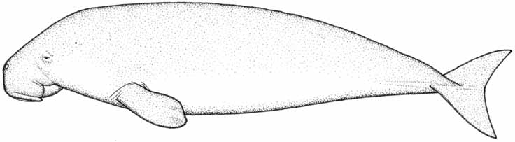
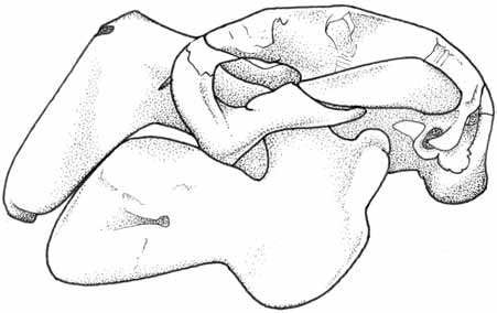
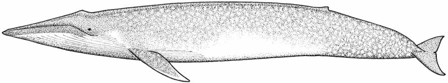
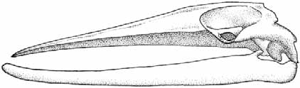
Standard Survey Methods
Appendix 9.6.3 Marine mammal guide to identification.
Dugong
Dugong dugon
Blue whale
Balaenoptera musculus
290

---

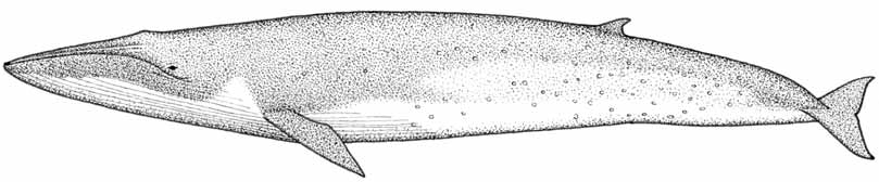
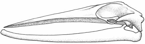
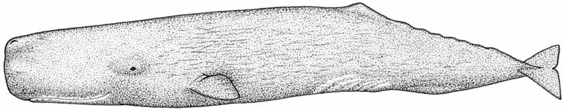
Marine Mammals
Bryde's whale
Balaenoptera edeni
Sperm whale
Physeter macrocephalus
291

---

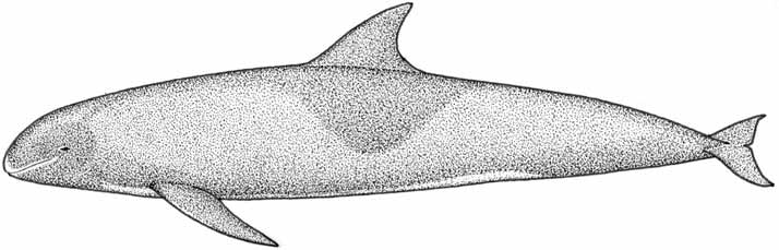
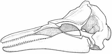
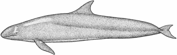
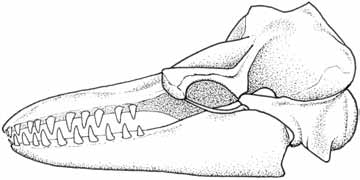
Standard Survey Methods
Melon­headed whale
Peponocephala electra
False killer whale
Pseudorca crassidens
292

---

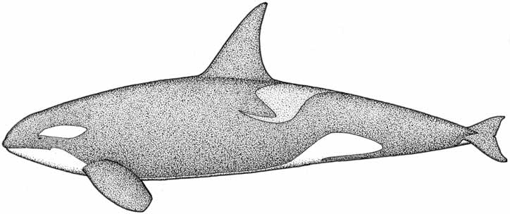
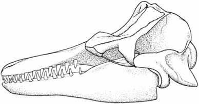
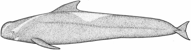
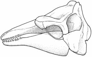
Marine Mammals
Killer whale
Orcinus orca
Short­finned pilot whale
Globicephala macrorhynchus
293

---

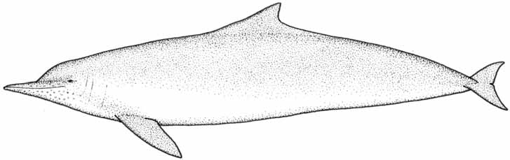
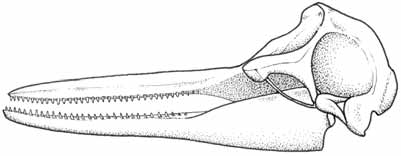
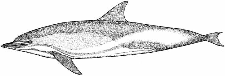
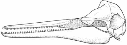
Standard Survey Methods
Indo­Pacific humpbacked dolphin
Sousa chinensis
Common dolphin
Delphinus delphis
294

---

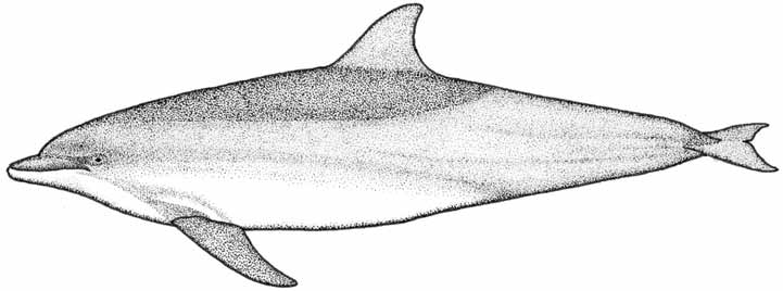
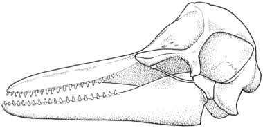
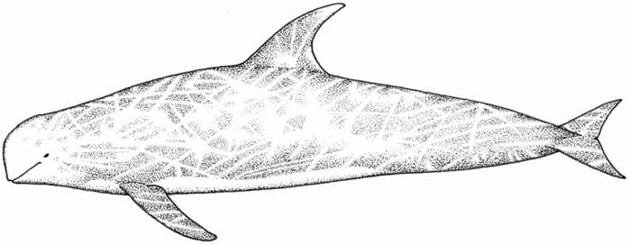
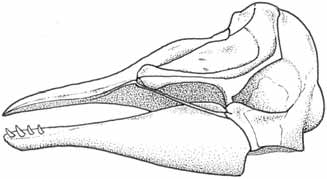
Marine Mammals
Bottlenose dolphin
Tursiops truncatus
Risso's dolphin
Grampus griseus
295

---

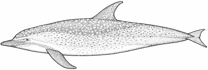
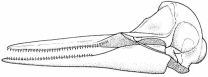
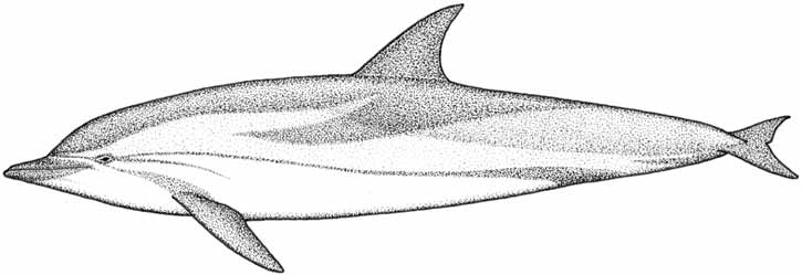
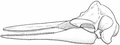
Standard Survey Methods
Pantropical spotted dolphin
Stenella attenuata
Striped dolphin
Stenella coeruleoalba
296

---

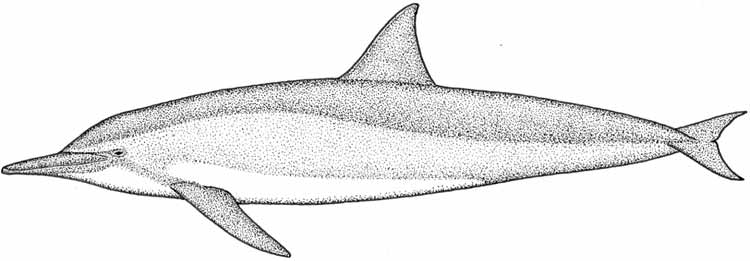
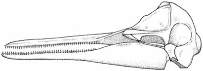
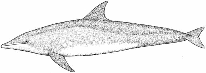
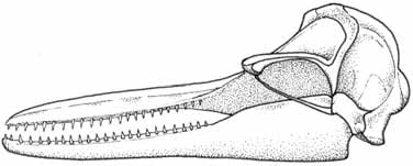
Marine Mammals
Spinner dolphin
Stenella longirostris
Rough­toothed dolphin
Steno bredanensis
297

---

Standard Survey Methods
Appendix 9.6.4
SIMPLE IDENTIFICATION GUIDE AND CARCASS DATA SHEET
(PREEN et al. 1989)
Information on the species, sex and size of these animals can provide useful information on the
structure, dynamics and health of the Red Sea marine mammal populations. Once a baseline of
data is collected, so that it is known at what rate animals normally die along the coast, the
incidence of stranding may prove a useful indicator of major pollution or disease events and
therefore an indicator of the health of the Red Sea generally.
Marine mammals can be identified by the following characteristics:
They have one or two blow-holes (nostrils) on top of their head through which they
breathe.
They have smooth skin (dugongs have very sparse fine hairs).
Their tail is flattened horizontally and it moves with an up-and-down motion. The tails
of fish are flattened vertically and move from side to side.
A description of four common marine mammal species occurring in the Red Sea and
the Gulf of Aden is given on the following page.
How to Measure Size and Determine Gender
The Figure 9.3 overleaf illustrates how to determine the sex and measure the length of a marine
mammal. Body length is the straight line distance (not curved) between the tip of the snout and
the notch of the tail fluke.
The sex of the marine mammal is determined by inspecting the relative distance between anus,
genital slit and navel scar on the belly of the animal. In females the genital slit is very close to
the anus, while in males the genital slit is more equidistant between the navel and the anus.
Data Sheet ­ Marine Mammal Carcass
A data sheet is given so that all observers may record their data in a standard format. The data
requested is the minimum necessary for the information to be useful.
Photographs
It is very helpful if photographs are taken of each dead animal. These photographs may provide
the specialist with information which could not be collected by the beach surveyor.
Dugongs
Dugong skulls are of particular scientific value and should be collected from carcasses
whenever possible.
Send data sheets, photos and skulls to:
PERSGA, P.O. Box 53662, Jeddah 21583, Kingdom of Saudi Arabia
298

---

Marine Mammals
DESCRIPTION OF FOUR COMMON MARINE MAMMAL SPECIES FROM THE RED
SEA AND GULF OF ADEN
Species:
Dugong
Scientific Name:
Dugong dugon
Body Length:
Up to 3 m
Dorsal fin:
No dorsal fin
Snout:
Blunt, enlarged, with coarse bristles on lower surface
Teeth:
2 to 5 large flattened teeth in the back of each jaw. In sexually mature males,
large incisors occur at the tip of the upper snout.
Colour:
Live:
Light brown to grey
Dead:
Dark brown to grey
Tail:
Large, without pronounced notch (which is characteristics of dolphins)
Teats:
1 to 4 cm long, just behind flippers.
Species:
Bottlenose dolphin
Scientific Name:
Tursiops truncatus
Body Length:
Up to 3.5 m
Dorsal fin:
High, curved backwards
Snout:
Short and stout
Teeth:
20 to 29 in each side of each jaw
Colour:
Live:
Grey back, light belly
Dead: Black
Species:
Common dolphin
Scientific Name:
Delphinus delphis
Body Length:
Up to 2.5 m
Dorsal Fin:
Very high, curved backwards
Snout:
Long and slender
Teeth:
45 to 57 in each side of each jaw
Colour:
Live:
Dark grey above, pale below, crisscross pattern of tan and grey on flanks
Dead: Black
Species:
Humpback dolphin
Scientific Name:
Sousa chinensis
Body Length:
Up to 3 m
Dorsal Fin:
Relatively small, curved backwards with rounded tip. Often set on an
elongated hump in the middle of the back.
Snout: Long
Colour:
Live:
Light to dark grey, sometimes speckled with darker spots
Dead: Black
299

---

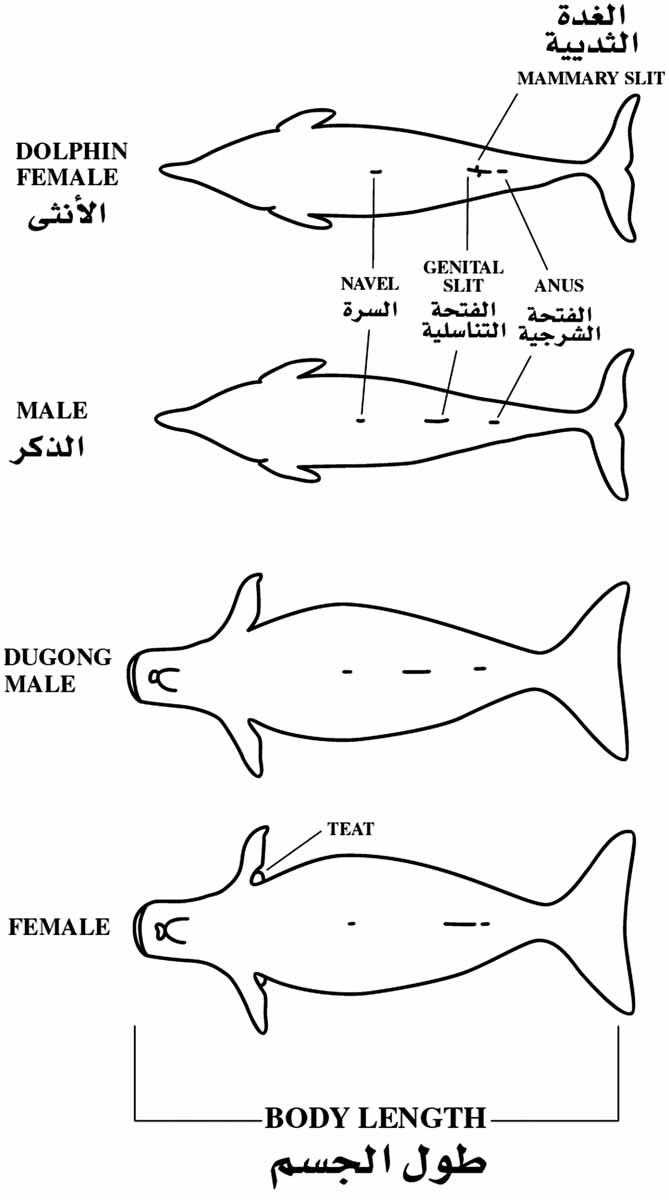
Standard Survey Methods










Figure 9.3 How to measure dolphin and dugong length and to determine sex
300

---

Marine Mammals
DATA SHEET ­ STRANDED MARINE MAMMAL CARCASS









:
________________________________________________________________
Date:

Name of Recorder:

:
_________________________________________________

Location of Carcass:

_____________________ (
:


)



___________________________________________________________________________
(Lat./Long.)________________________________________________________________
Species:

:
______________________________________________________________
Sex: Male / Female / Could not tell












/
/
:

Body Length: _____ Metres
:
____________________


Photos Taken: Yes/No?


/
:


Skull Collected: Yes/No?


/
:




Where is the skull now?
:
_________________________________________


___________________________________________________________________________
Comments:
:
_________________________________________________________
___________________________________________________________________________

:
Address and Telephone Number of Recorder
:
______
__________________


___________________________________________________________________________


Please send data sheets, photos and skulls to:

PERSGA, P.O. Box 53662, Jeddah 21583, Kingdom of Saudi Arabia

301

---

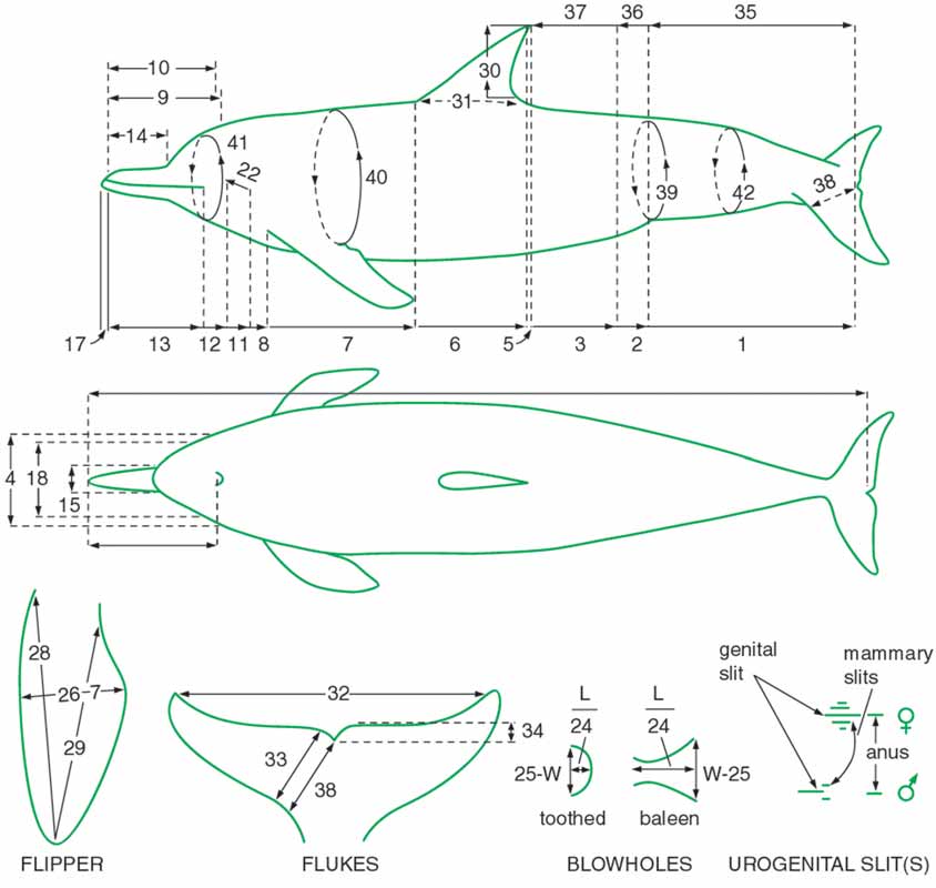
Standard Survey Methods
Appendix 9.6.5 Cetacean data record schematic.
Locations and details of important measurements
Figure 9.4 Schematic for collecting morphometric data from cetaceans (LEATHERWOOD et al. 1976)
302

---

Marine Mammals
CETACEAN DATA RECORD
SPECIES________________________SEX_______LENGTH________WEIGHT___________
DATE/TIME STRANDED____________________ DATE/TIME COLLECED _____________
LOCATION OF COLLECTION __________________________________________________
OBSERVER NAME / ADDRESS _________________________________________________
SPECIMEN SENT TO __________________________________________________________
Straight line parallel
to the body axis
Point to Point
MEASUREMENTS:
1.
Tip of upper jaw to deepest part of fluke notch
_____________ ____________
2.
Tip of upper jaw to centre of anus
_____________
____________
3.
Tip of upper jaw to centre of genital slit
_____________
____________
4.
Tip of lower jaw to end of ventral grooves
____________
5.
Tip of upper jaw to centre umbilicus
_____________
____________
6.
Tip of upper jaw to top of dorsal fin
_____________
____________
7.
Tip of upper jaw to leading edge of dorsal fin
_____________
8a.
Tip of upper jaw to anterior insertion of flipper (right)
_ ____________
____________
b.
Tip of upper jaw to centre of blowhole(s)
_____________
____________
10. Tip
of
upper jaw to anterior edge of blowhole(s)
_____________ ____________
11a.
Tip of upper jaw to centre of eye (right)
_____________
____________
b. Tip of upper jaw to centre of eye (left)
_____________
____________
12a.
Tip of upper jaw to centre of eye (right)
_____________
____________
b. Tip of upper jaw to centre of eye (left)
_____________
____________
13.
Tip of upper jaw to angle of gape
____________
14.
Tip of upper jaw to apex of melon
_____________
15.
Rostrum ­ maximum width
_____________
____________
16.
Throat grooves ­ length
_____________
____________
17.
Projection of lower jaw beyond upper (if reverse, so state) ___________
18.
Centre of eye to centre of eye
____________
19a.
Height of eye (right)
_____________
b. Height of eye (left)
_____________
20a.
Length of eye (right)
_____________
b. Length of eye (left)
_____________
21a.
Centre of eye to angle of gape (right)
_____________
____________
b. Centre of eye to angle of gape (left)
_____________
_____________
22a.
Centre of eye to external auditory meatus (right)
_____________
____________
b. Centre of eye to external auditory meatus (left)
_____________
____________
303

---

Standard Survey Methods
Straight line parallel
to the body axis
Point to Point
23a.
Centre of eye to centre of blowhole (right)
_____________
_____________
b. Centre of eye to centre of blowhole (left)
_____________
_____________
24.
Blowhole length
_____________
25.
Blowhole width
_____________
26.
Flipper width (right)
_____________
27.
Flipper width (left)
_____________
28a.
Flipper length ­ tip to anterior insertion (right)
_____________
b. Flipper length ­ tip to anterior insertion (left)
_____________
29a.
Flipper length ­ tip to axilla (right)
_____________
b. Flipper length ­ tip to axilla (left)
_____________
30.
Dorsal fin height
_____________
31.
Dorsal fin base
_____________
32.
Fluke span
_____________
33.
Fluke width
_____________
34.
Fluke depth of notch
_____________
35.
Notch of flukes to centre of anus
_____________
_____________
36.
Notch of flukes to centre of genital aperture
_____________
37.
Notch of flukes to umbilicus
_____________
38.
Notch of flukes to nearest point on leading edge of flukes ___________
39.
Girth at anus
_____________
40.
Girth at axilla
_____________
41.
Girth at eye
_____________
42.
Girth ____cm in front of notch of flukes
_____________
43a.
Blubber thickness (mid dorsal)
_____________
b. Blubber thickness (lateral)
_____________
c. Blubber thickness (mid ventral)
_____________
44.
Width of head at post-orbital process of frontals
_____________
45.
Tooth count: right upper
__________
right lower
__________
left lower
__________
46.
Baleen count:
right upper
__________
left upper
__________
47.
Baleen plates, length longest
_____________
48.
Baleen plates, no. bristles/cm over 5 cm
_____________
49a.
Mammary slit length (right)
_____________
b. Mammary slit length (left)
_____________
50.
Genital slit length
_____________
51.
Anal slit length
_____________
304

---

Marine Mammals
Appendix 9.6.6
DUGONG CARCASS DATA SHEET
Specimen Number: ________
Examined by: ____________________________________________
Contact Address:__________________________________________
Location: ______________________________________________________________________
Date of examination: __________ Time: ________ Estimated time since death: ______________
Condition: live/ fresh dead / fair / bloated / collapsed
Photos taken? Yes / No
External marks (bites, nets, etc.) _________________________________________________
Body length (see illustration) ______ _____________ m
Length of teats: Left ________cm Right _________ cm
Gender (see illustration): Male / Female
Tusks present: Yes/ No
NOTE: This is hierarchy of observations, proceed as far as you feel competent.
Comments on external features:
Skin__________________________________________________________________________
Eyes__________________________________________________________________________
Nostrils _______________________________________________________________________
Flippers _______________________________________________________________________
Tail Fluke _____________________________________________________________________
General physical condition: good / poor
Foetus present?
Length_______ Gender _______ Weight _________
Milk being produced? (cut mammary gland) ______________
305

---

Standard Survey Methods
Comments on internal organs:
Body-wall fat:
firm & white / yellow, jelly-like & watery
Stomach:
full / half full / less
Intestines:
packed with food / relatively empty
external colour: white / yellow / pink / red / other
Liver:
colour ________________
edge profile: rounded/ sharp
Respiratory Tract:
Trachea:
internal colour: white / pink/ red / other
Lungs:
colour: pink / red / other___________
Texture: soft / firm
Heart:
colour of surrounding fat: yellow / white / other
Possible Samples (label fully)
Organ
Preparation
Analyses
Body fat
Freeze
Toxins, Heavy Metals
Blood
Anti­coagulant
Red cell count
No anti­coagulant
Blood chemistry
Skin
Freeze
Genetics
Stomach content
Freeze/formalin*
Diet, toxic dinoflagellates
Liver
Freeze
Toxins
Gall bladder
Freeze
Toxins
Gonads
Formalin/freeze
Reproductive history
Skull
Freeze/deflesh
Age
* 10% seawater formalin (9 parts seawater to 1 part formalin)
Comments:
______________________________________________________________________________
______________________________________________________________________________
______________________________________________________________________________
306

---

Marine Mammals
e










Photos










Roll Fram
ave
ter depth)
a
Conditions
, visibility, w
Environmental
height, w
(
wind





















at

Position of Boat
time of sighting
Lat. Long.










e
Siz
.
(estimate)











Behaviour Group











Method of











Observation
(eye or 7x,
20x bino.)
om a line-transect boat survey











Features
Species Diagnostic











r
ecording information fr











boat
Bearing &
Distance from
deg. (m)

24:00
Time of
Sighting
No.










Date:.................................................... Name of Recorder:..................................
Name of boat:.......................................... Skipper:..................................... Name of Observer:.................................

Sighting


Appendix 9.6.7 Data sheet for
307

---

Standard Survey Methods
Appendix 9.6.8
Data sheets for aerial transect survey.
FLIGHT SUMMARY SHEET
Date:_____________
Aircraft:___________________________
Controller/Recorder:_______________
Pilot: _____________________________
Observer Left Front:________________
Observer Right Front:________________
Observer Left Rear: ________________
Observer Right Rear: ________________
Location start: ____________________
Location end: ______________________
Engine start:_____________ Engine shut-down:______________ Diff.: __________
Altimeter start:___________ Altimeter end: _________________ Diff.: __________
Survey conditions:________________________________________________________
_______________________________________________________________________
Transects flown (in order): _________________________________________________
_______________________________________________________________________
Notes:__________________________________________________________________
_______________________________________________________________________
_______________________________________________________________________
_______________________________________________________________________
308

---

Marine Mammals
TRANSECT DATA SHEET
Date:
Transect #:
Trn start:
Trn end:
Time
Alt
Beauf Glare
Obs
Sp.
Grp
# at
Posn
#
Species
ID
type
size
surf
in
calves
cert
Trn
Trn. start:
exact start times of the transect.
Trn. end:
exact end times of the transect.
Time:
exact time of sighting/record.
Alt.:
aircraft altitude read from altimeter. Ensure several records per transect.
Beauf.:
sea state using Beaufort scale. Ensure several records per transect.
Glare:
a measure of the proportion of the search area affected by glare from the sun. The following
scale is suggested: 0 = no affect of glare, 1 = up to 25% of search area affected by glare, 2 = up
to 50% of search area affected, 3 = >50% search area affected by glare. Request a glare reading
from observers several times during each transect.
Obs.:
observer
Sp. type:
type of animal or object. Use a unique code for each category e.g. D = dugong, C = cetacean,
T = turtle, S = shark, R = ray, B = birds, W = whale shark, V = vessel, N = net.
Grp. size:
number of animals/objects in sighting group within transect.
# at surf:
number of animals within the group that are breaking the water surface. This information is
needed for the Availability correction factor.
Posn. in Trn.:
position of sighting within the transect (H = high, M = mid, L = low). Important where there
are front and rear-seat observers to determine if near simultaneous sightings are of the same or
different animals/objects.
# calves:
number of calves in the group.
Species:
more specific identification of species type. Develop unique codes for the types of cetaceans
expected in the area. May also need codes for rays (manta, eagle, sting), seabirds, vessels and
nets.
ID cert.:
Confidence of species identification; this is particularly important for cetaceans. C= certain,
P = probable, G = guess.
309

---

Standard Survey Methods
310

---