Seamounts are hotspots of pelagic biodiversity in the
open ocean
Telmo Moratoa,b,1, Simon D. Hoylea, Valerie Allaina, and Simon J. Nicola
aOceanic Fisheries Program, Secretariat of the Pacific Community, BPD5 98848 Noumea, New Caledonia; and bDepartamento de Oceanografia e Pescas,
Universidade dos Açores, 9901-862 Horta, Portugal
Edited by David Karl, University of Hawaii, Honolulu, HI, and approved April 13, 2010 (received for review October 6, 2009)
The identification of biodiversity hotspots and their management
to seamounts to identify those pelagic species that are signifi-
for conservation have been hypothesized as effective ways to
cantly associated with seamounts. The dataset comprised a time
protect many species. There has been a significant effort to
series from 1980 to 2007 of species catch data collected on tuna
identify and map these areas at a global scale, but the coarse
longline vessels by independent observers over large areas of the
resolution of most datasets masks the small-scale patterns asso-
western and central Pacific Ocean, coupled with comprehensive
ciated with coastal habitats or seamounts. Here we used tuna
data on the location of seamounts (24).
longline observer data to investigate the role of seamounts in
aggregating large pelagic biodiversity and to identify which
Results
pelagic species are associated with seamounts. Our analysis
Seamounts as Hotspots of Biodiversity? Rarefied pelagic diversity
indicates that seamounts are hotspots of pelagic biodiversity.
was significantly higher in seamount habitats than in coastal or
Higher species richness was detected in association with sea-
oceanic waters (Fig. 1A) and was found to be nonlinearly related
mounts than with coastal or oceanic areas. Seamounts were found
to the distance to seamount, with diversity higher close to the
to have higher species diversity within 30­40 km of the summit,
summits (Fig. 1B). Rarefied diversity was higher at intermediate
whereas for sets close to coastal habitat the diversity was lower
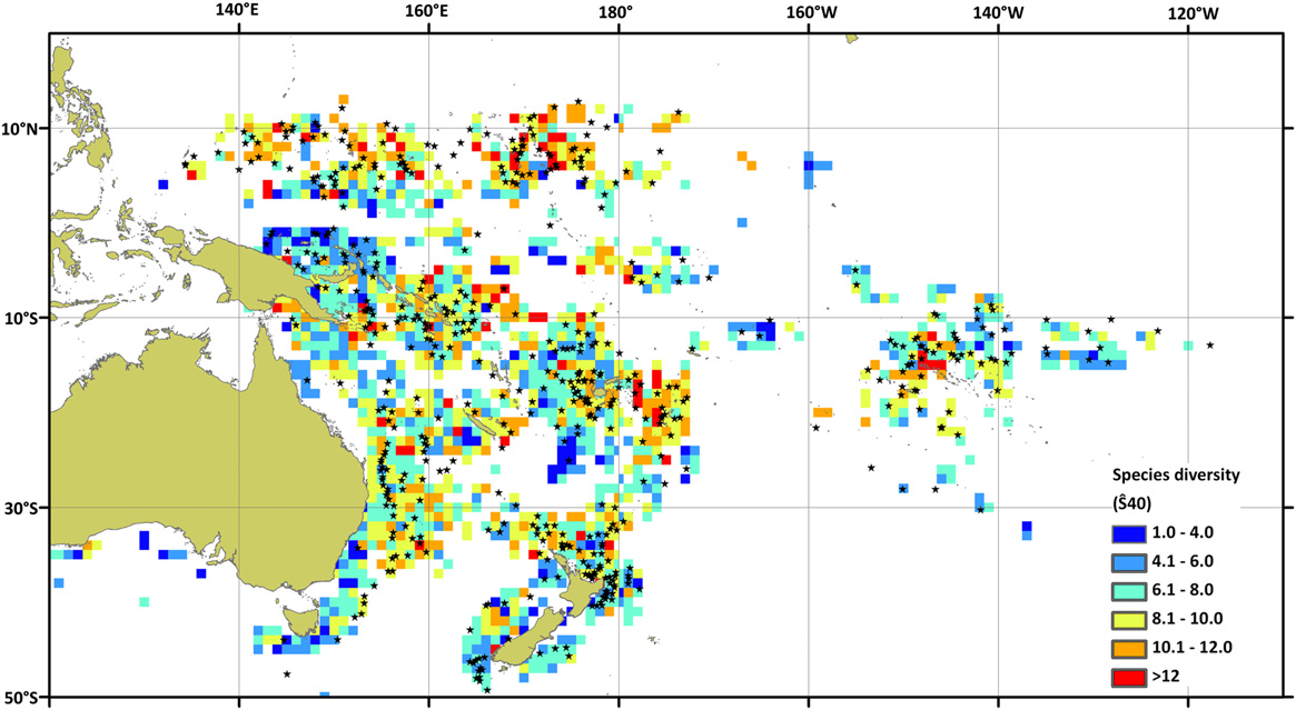
latitudes (10­35 °S and 10­15 °N; Fig. 1C). Regions with higher
ENTAL
and fairly constant with distance. Higher probability of capture
pelagic diversity included Indonesia, Palau, Federated States of
and higher number of fish caught were detected for some shark,
Micronesia, and Marshall Islands in the Northern Hemisphere
SCIENCES
billfish, tuna, and other by-catch species. The study supports hy-
and Tonga, New Caledonia, and Norfolk Island in the Southern
ENVIRONM
potheses that seamounts may be areas of special interest for man-
Hemisphere (Fig. 2). The relationship for describing species di-
agement for marine pelagic predators.
versity was complex with distance to features, number of hooks,
and latitude the strongest predictors of species diversity (Table
by-catch | fisheries | longline | pelagic predators | seamount conservation
1). When all variables except distance to feature were kept
constant, seamounts were found to have higher rarefied diversity
For the last decade there has been considerable debate about within 30­40 km of the summit (Fig. 3). For coastal and oceanic
the status and sustainability of pelagic fisheries around the
habitats the rarefied diversity was lower and not affected by
world (1­6) and their effects on the ecosystems that support
distance to the feature (Fig. 3). A statistically significant effect of
them (7­10). Many species may be protected by identifying
moon was not detected for rarefied diversity. The detailed GLM
biodiversity hotspots and managing them for conservation (11).
results are presented in Table S1.
This approach is well established for terrestrial systems and
marine tropical reefs (12, 13), but less so for the pelagic eco-
Highly Migratory Pelagic Species Aggregating Around Seamounts. To
identify which species aggregate around seamounts, the re-
systems of the open ocean (11). Simulation modeling has in-
lationship between CPUE and distance to seamounts was ex-
dicated that management techniques such as area closure are
amined for individual species. There were sufficient data to
likely to help conserve many pelagic species (11). Accordingly,
analyze 37 taxa. Of these, seamount aggregation effects were
there has been a significant effort to identify and map pelagic
detected for 41% of the taxa (15 taxa of shark, billfish, and pe-
biodiversity hotspots at a global scale, but progress has been
lagic teleost fish), although the opposite effects were detected for
limited. The coarse resolution of most datasets masks the small-
only 3 taxa (Table 2). For the shark taxa the probability of
scale patterns associated with coastal habitats or seamounts (14).
catching the species increased closer to seamounts for porbeagle
Hotspots that have been identified in open ocean areas have
shark (Lamna nasus), short-finned mako shark (Isurus oxy-
been typically associated with particular environmental factors
rinchus), and silky shark (Carcharhinus falciformis) and de-
and mesoscale oceanographic features such as latitude, fronts, or
creased for pelagic stingray (Pteroplatytrygon violacea). The
eddies (14, 15). The dynamism of pelagic environments can
average number caught per set was also higher closer to sea-
significantly reduce the efficacy of conservation measures (16).
mounts for silky sharks. We did not detect an effect of seamount
To address this issue, dynamic marine reserves that move with
on the probability of being caught for blue shark (Prionace
the wildlife have been suggested (17), but such approaches may
glauca), but observed that in sets that caught the taxa the average
not be workable (18).
number caught was higher closer to seamounts. For the billfishes
Many seamounts are important aggregating locations for
and tunas the probability of catching the species increased closer
highly migratory pelagic species (19­23), but their role in ag-
to seamounts for yellowfin tuna (Thunnus albacares), blue marlin
gregating pelagic biodiversity is largely unknown. If seamounts
are hotspots for pelagic biodiversity then they may prove to be
suitable areas for conservation measures in open ocean envi-
Author contributions: T.M., V.A., and S.J.N. designed research; T.M., V.A., and S.J.N. per-
ronments. Morato et al. (23) demonstrated that seamounts ag-
formed research; S.D.H. contributed new reagents/analytic tools; T.M. and S.D.H. analyzed
gregate some visitor species but did not demonstrate that this
data; and T.M., S.D.H., V.A., and S.J.N. wrote the paper.
behavior can be generalized. Building upon this previous work,
The authors declare no conflict of interest.
we examine the role of seamounts in aggregating pelagic bio-
This article is a PNAS Direct Submission.
diversity by applying ocean basin scale generalized linear models
1To whom correspondence should be addressed. E-mail: t.morato@gmail.com.
(GLMs) to location-specific fisheries catch data. In addition, we
This article contains supporting information online at www.pnas.org/lookup/suppl/doi:10.
analyzed catch per unit of effort (CPUE) in relation to distance
1073/pnas.0910290107/-/DCSupplemental.
www.pnas.org/cgi/doi/10.1073/pnas.0910290107
PNAS Early Edition | 1 of 5

---

A
B
C
7.0
8.0
8.5
6.9
7.8
8.0
7.6
6.8

40)
(
7.4
7.5
6.7
sity 6 6
7.2
7.0
6.6
7.0
6.5
6.5
Diversity
6.8
6.0
6.4
6.6
6.3
5.5
Species
6.4
6.2
5.0
6.2
R²
R² = 0.81
6.1
6.0
4.5
SM
Shore
Oceanic
0
20
40
60
80
100
-55 -45 -35 -25 -15 -5
5 15
Habitat
Distance to seamount summit (km)
La tude
Fig. 1.
Mean expected species diversity (±95% confidence limits) rarefied from 40 individuals (^
S40) as a function of (A) the main habitat [seamount (SM),
shore and oceanic] where all means are significantly different at = 0.01 (ANOVA and Tukey's honestly significant difference test), (B) distance to seamount
summit where the fitted logarithmic regression is also shown (shaded line), and (C) 5 ° latitude.
(Makaira nigricans), and swordfish (Xiphias gladius) and de-
gregation effects on both probability of capture and number
creased for albacore (Thunnus alalunga) and shortbill spearfish
caught were also observed for the unidentified species category.
(Tetrapturus angustirostris). For the other pelagic teleost fish the
Discussion
probability of catching the species increased closer to seamounts
for ribbon fish (Trachipterus trachypterus), butterfly kingfish
Our analyses suggest that seamounts are hotspots of pelagic
(Gasterochisma melampus), big-scaled pomfret (Taractichthys
biodiversity, because they show consistently higher species rich-
ness than do shore or oceanic areas. Moreover, our study indi-
longipinnis), Atlantic pomfret (Brama brama), and long-snouted
cates that higher species diversity is likely to occur within 30­40
lancetfish (Alepisaurus ferox). The average number caught per
km of seamount summits. This study also demonstrates that
successful set was also higher closer to seamounts for butterfly
many marine predators and other visitors are associated with
kingfish but lower for ribbon fish and big-scaled pomfret. We did
seamounts. The GLM model did not take into account the
not detect an effect of seamount on the probability of being
species being targeted or the depth and time of sets as in-
caught for short-snouted lancetfish (Alepisaurus brevirostris) and
formation on these variables was not contained within the da-
moonfish (Lampris guttatus), but observed that the average
tabase. These factors may influence the results but are unlikely to
numbers caught per successful set were higher closer to sea-
affect the overall patterns, which are robust.
mounts for both species. For the other 19 species, statistically
Associations with seamounts have been previously described
significant trends were not detected (Table S2). Seamount ag-
for a few species of tuna (20, 23, 25, 26), sharks (22, 27), billfishes
Fig. 2.
Expected species diversity rarefied from 40 (^
S40) individuals as a function of 1 × 1 degree cells. Stars denote locations of seamounts with longline sets
close to their summits.
2 of 5 | www.pnas.org/cgi/doi/10.1073/pnas.0910290107
Morato et al.

---

Table 1.
Summary statistics for the GLM single-variable
survey, and enforce. The establishment of a network of marine
elimination analyses relating species diversity with habitat and
reserves on seamounts may help to conserve pelagic biodiversity
other variables
and achieve sustainability of marine predator species, such as
porbeagle shark, short-finned mako shark, silky shark, blue
df
Deviance
AIC
P
shark, yellowfin tuna, blue marlin, swordfish, ribbon fish, but-
49,748
54,383
terfly kingfish, big-scaled pomfret, Atlantic pomfret, long-
Year
22
50,977
54,654
<0.001
snouted lancetfish, short-snouted lancetfish, and moonfish.
Moon
7
49,792
54,380
0.133
Month
11
49,939
54,410
<0.001
Materials and Methods
Lat5
12
52,747
55,115
<0.001
Fisheries and Seamount Data. The Western and Central Pacific Ocean (WCPO)
Long5
26
50,793
54,599
<0.001
is by far the most important tuna fishing ground in the world, contributing
Flag_Fleet
29
51,295
54,720
<0.001
50% (2.4 million tons in 2007) of the global tuna catches (38) at an eco-
nomic value of US$3.8 billion. The longline fishery in the WCPO has a smaller
EEZ
21
50,848
54,623
<0.001
catch (10% of the total), but its value is relatively high (30% of the total
Hooks (ns, df = 10)
10
56,736
56,061
<0.001
value). It targets adult bigeye (Thunnus obesus), yellowfin (T. albacares), and
log(dist.) × feature
2
49,807
54,394
<0.001
albacore tuna (T. alalunga), and in some cases sharks or swordfish (X. gla-
dius), and operates with fairly standard gear con
AIC, Akaike
figurations that comprise
's information criterion; df, degrees of freedom; EEZ, Exclusive
a main line, branch lines between
Economic Zone; ns, natural cubic splines.
floats, and float lines. The Secretariat of
the Pacific Community (SPC) maintains the regional database for fisheries
observer programs in the WCPO, which commenced in 1980. The study area
(28, 29), some seabirds (23, 30), and some marine mammals (23,
extends from 35 °N to 50 °S in latitude and from 130 °E to 120 °W in lon-
gitude (Fig. S1). All longline sets from the period 1980­2007 were extracted
31), mostly at an individual seamount scale. Our study suggests,
from the SPC's observer dataset, which include trips conducted onboard
however, that seamount associations are probably more common
industrial and semi-industrial vessels from the Pacific Island Countries and
and widespread than previously anticipated. The resolution of
Territories and from distance-water fishing nations. Depth of fishing was not
the data collected does not provide any opportunity to identify
recorded but is known to vary according to setting strategies. The database
the mechanistic explanations for why seamounts aggregate bio-
contains 23,546 longline sets with the number of hooks per set ranging from
ENTAL
diversity. However, seamounts generate conditions such as in-
a few hundred to several thousand, averaging 2,000 hooks per set. Ob-
creased vertical nutrient fluxes and material retention that
server quality was assumed to be consistent across all sets. The dataset
SCIENCES
promote productivity and fuel higher trophic levels (32­34).
contains catch data for 352 taxa, but only 50 taxa were recorded in >500
ENVIRONM
longline sets (Table S3). The number of recorded species as a function of
Seamounts also have unique "magnetic signatures" that may
fishing effort reached an asymptote (at 10­20 million hooks), indicating
contribute to their use as rest stops or feeding grounds for many
that the sample size obtained from the observer programs was sufficient to
pelagic species such as sharks, whales, and other migrants (35,
perform the biodiversity analyses (Fig. S2).
36). It is likely that the mechanistic explanation is a combination
Catch by species was returned as number, size, and weight. Date and
of factors that make seamounts suitable mating, feeding, and
geographic location of the set, number of hooks, and flag and fleet of the
nursery grounds for highly migratory pelagic species as well as
fishing boat were also extracted. The distance of each longline set to the
benthic organisms (37).
closest seamount was estimated using the simple spherical law of cosines and
Higher pelagic biodiversity has previously been noted in in-
a Pacific seamount dataset containing 7,741 features (24, 39). Additionally,
distances of longline sets to the closest shore were estimated using a land
termediate latitudes (11) and our analyses support this hypoth-
shapefile (including atolls). Longline sets were then categorized by habitat
esis. However, we also noted high diversity in some tropical
as seamount sets (distance to seamount < distance to shore and < 100 km),
latitudes. In previous studies, data have been scarce for the
coastal sets (distance to shore < distance to seamount and < 100 km), or
tropical latitudes between 10 °N and 10 °S, whereas the observer
oceanic sets (distance to shore and distance to seamount >100 km). The
data used in this study provided more comprehensive coverage.
longline dataset contained 10,602 seamount sets, 5,164 coastal sets, and
Further development of observer programs to ensure compre-
7,780 oceanic sets.
hensive spatial and temporal coverage is encouraged.
Conserving biodiversity hotspots has been demonstrated to
Biodiversity Analyses. Species richness is known to increase with sample size,
and differences in richness may be caused by differences in sample size. To
yield significant conservation benefits (11). Therefore, our
solve this problem, we used rarefaction techniques to account for differences
analyses support the utility of seamounts as potential locations
in fishing effort (number of hooks) among longline sets (40, 41). The
for offshore marine reserves. Seamount habitats are easier to
expected number of species (^
S40), standardized to 1,000 hooks per longline
conserve than ephemeral areas because they are easier to map,
set, was rarefied for subsamples of 40 individuals from the total number of
Fig. 3.
The effect of the variables distance × feature on species diversity rarefied from 40 individuals (^
S40). One variable was predicted at a time from the
results of the GLM by fixing the other variables.
Morato et al.
PNAS Early Edition | 3 of 5

---

Table 2.
Statistics for all by-catch species that were observed in >500 of 10,602 sets (n > 500),
for both the binary and the lognormal components of the GLM
Binary
Lognormal
Species
N
AIC
LogdistSM
SM effect
AIC
LogdistSM
SM effect
Sharks and Rays
Blue shark
7,115
1.84
0.0153
-4.34
-0.0431
Higher
Porbeagle shark
1,572
-5.40
-0.1976
Higher
1.28
0.0262
Silky shark
1,890
-1.20
-0.0954
Higher
-1.92
-0.0591
Higher
Pelagic stingray
2,116
-5.18
0.1149
Lower
0.82
0.0241
Short-finned mako shark
2,207
-4.62
-0.1111
Higher
0.69
0.0199
Billfishes and similar
Swordfish
3,973
-1.21
-0.0668
Higher
0.76
-0.0178
Blue marlin
1,977
-2.36
-0.0936
Higher
0.63
0.0214
Shortbill Spearfish
1,451
-4.75
0.1405
Lower
2.00
-0.0013
Tuna, bonito and mackerel
Albacore
6,898
-2.64
0.1164
Lower
-12.50
0.0662
Lower
Yellowfin
6,420
-3.12
-0.1095
Higher
1.88
0.0068
Pelagic fish and others
Longsnouted lancetfish
3,268
-2.46
-0.0859
Higher
1.53
0.0143
Atlantic pomfret
2,365
-2.22
-0.1077
Higher
0.95
-0.0322
Moonfish
3,065
0.49
-0.0465
-0.24
-0.0258
Higher
Big-scaled pomfret
892
-5.62
-0.1694
Higher
-2.46
0.0678
Lower
Butterfly kingfish
1,013
-5.46
-0.1848
Higher
-8.94
-0.0980
Higher
Ribbon fish
577
-5.85
-0.3128
Higher
-0.94
0.0956
Lower
Short-snouted lancetfish
741
1.34
-0.0511
-0.37
-0.0575
Higher
Unidentified taxa
1,603
-0.77
-0.0810
Higher
-0.53
-0.0504
Higher
For each component we present the effect of including the term for distance to seamount on the AIC (AIC),
the parameter estimate for the relationship with log(distance to seamount), and whether the effect represents
a significantly higher or lower catch rate close to seamounts (SM). Only those taxa with statistically significant
trends are shown here. The complete table is shown in Table S2.
individuals in the sample. This methodology has been extensively used to
and was within 100 km (Fig. S3). We modeled the data in two parts using a -
compare the species richness obtained from longline fishing fleets (11, 14,
lognormal GLM (44). In the first (binomial) part we modeled the probability
42). The effects of habitat type and distance to habitat feature were ana-
of catching any of the species in a set. In the second (lognormal) part we
lyzed for the estimated rarefied richness.
modeled the number caught in sets where at least one animal was caught.
GLM techniques were used to standardize rarefied richness and to eval-
We used AIC to test for effects of distance to seamount by modeling the
uate whether the presence of habitat features and the distance to the feature
data with and without a seamount term. The explanatory variables included
were significant explanatory variables. The explanatory variables included in
in the models were the same as in the biodiversity analyses. The models
the model were year as a proxy for temporal variability, moon phase as the
adopted to standardize data were
relationship between lunar periodicity and catch rates as has been demon-
strated for a wide variety of commercially exploited species (e.g., ref. 43),
Logit½pðspecies 0Þ year þ moon phase þ month þ lat5 þ long5
geographical area, fleet type, distance to the closest feature, and fishing
n
effort. Akaike's information criterion (AIC) was used to compare the model
þ flagfleet þ hooks þ LogðdistSMÞ;
fits using different relationships with distance to feature, with log-trans-
formed having the better fit. The model used was
where speciesn 0, and
^S40 ~ Year þ moon phase þ month þ lat5 þ long5
þ

flagfleet þ Logðdistance to featureÞ· feature
speciesn year þ moon phase þ month þ lat5 þ long5 þ flagfleet
þ
þ
nsðhooks; df ¼ 10Þ:
hooks þ LogðdistSMÞ:
Years included in the standardization were 1982 and 1987­2007 because ^
S40
estimates were not available for other years. Moon phase was divided into
We examined the residuals to check that the assumptions were not vi-
eight categories from new to full. The geographical areas used in the
olated for each model. By-catch species were considered to be associated
standardization were squares of 5 ° latitude and longitude because they
with seamounts if the seamount distance effect was statistically sig-
originate better fit than many other approaches. Vessels were categorized
nificant and negative (i.e., higher catch rate when closer to sea-
on the basis of a combination of their flag and fleet type. Effort was mea-
mount summits).
sured as the natural cubic splines (ns) of the number of hooks in each
longline set. The species being targeted and the depth and time of a set can
ACKNOWLEDGMENTS. We thank Nick Davies and Michael Manning for help
influence the nontarget species caught. Information on these variables was
with the modeling and Emmanuel Schneiter, Colin Millar, and Peter Williams
not contained within the database and fleet type and number of hooks
for help with the Observer database. We thank the two anonymous
were used as a proxy measures for these variables.
reviewers for their comments, which greatly improved the manuscript. We
acknowledge the Secretariat of the Pacific Community member countries for
the collection and provision of observer data. We particularly acknowledge
Analyses of the GLMs for Each Highly Migratory Pelagic Species. We used GLM
the important work done by the national observer programs throughout the
techniques to standardize catch data for each by-catch species caught in at
region. This research is part of the Pacific Islands Oceanic Fisheries
least 500 sets of the 10,602 sets for which a seamount was the closest feature
Management Project supported by Global Environment Facility.
4 of 5 | www.pnas.org/cgi/doi/10.1073/pnas.0910290107
Morato et al.

---

1. Baum JK, et al. (2003) Collapse and conservation of shark populations in the
25. Klimley AP, Jorgensen SJ, Muhlia-Melo A, Beavers SC (2003) The occurrence of
Northwest Atlantic. Science 299:389­392.
yellowfin tuna (Thunnus albacares) at Espiritu Santo Seamount in the Gulf of
2. Myers RA, Worm B (2003) Rapid worldwide depletion of predatory fish communities.
California. Fish Bull (Wash DC) 101:684­692.
Nature 423:280­283.
26. Rodríguez-Cabello C, Sánchez F, Ortiz de Zárate V, Barreiro S (2009) Does Le Danois
3. Hampton J, Sibert JR, Kleiber P, Maunder MN, Harley SJ (2005) Fisheries: Decline of
Bank (El Cachucho) influence albacore catches in the Cantabrian Sea? Cont Shelf Res
Pacific tuna populations exaggerated? Nature 434:E1­E2.
29:1205­1212.
4. Hilborn R (2006) Faith-based fisheries. Fisheries 31:554­555.
27. Klimley AP, Richard JE, Jorgensen SJ (2005) The home of blue water fish. Am Sci 93:
5. Sibert J, Hampton J, Kleiber P, Maunder M (2006) Biomass, size, and trophic status of
top predators in the Pacific Ocean. Science 314:1773­1776.
42­49.
6. Langley A, et al. (2009) Stock assessment of yellowfin tuna in the western and central
28. Sedberry GR, Loefer JK (2001) Satellite telemetry tracking of swordfish, Xiphias
Pacific Ocean. Western Central Pacific Fisheries Commission, Scientific Committee, 5th
gladius, off the eastern United States. Mar Biol 139:355­360.
Regular Session (Western Central Pacific Fisheries Commission, Port Villa, Vanuatu).
29. Poisson F, Fauvel C (2009) Reproductive dynamics of swordfish (Xiphias gladius) in the
Available at: http://www.wcpfc.int/system/files/documents/meetings/scientific-committee/
southwestern Indian Ocean (Reunion Island). Part 2: Fecundity and spawning pattern.
5th-regular-session/stock-assessment-swg/working-papers/SC5-SA-WP-03%20%
Aquat Living Resour 22:59­68.
5BYFT%20Assessment%20%28rev.1%29%5D.pdf.
30. Amorim P, et al. (2009) Spatial variability of seabird distribution associated with
7. Pauly D, Christensen V, Dalsgaard J, Froese R, Torres F, Jr (1998) Fishing down marine
environmental factors: A case study of marine Important Bird Areas in the Azores.
food webs. Science 279:860­863.
ICES J Mar Sci 66:29­40.
8. Jackson JBC, et al. (2001) Historical overfishing and the recent collapse of coastal
31. Parrish FA (2009) Do monk seals exert top-down pressure in subphotic ecosystems?
ecosystems. Science 293:629­638.
Mar Mamm Sci 25:91­106.
9. Worm B, et al. (2006) Impacts of biodiversity loss on ocean ecosystem services. Science
32. Genin A, Dayton PK, Lonsdale PF, Spiess FN (1986) Corals on seamounts provide
314:787­790.
evidence of current acceleration over deep sea topography. Nature 322:59­61.
10. Baum JK, Worm B (2009) Cascading top-down effects of changing oceanic predator
33. Lueck RG, Mudge TD (1997) Topographically induced mixing around a shallow
abundances. J Anim Ecol 78:699­714.
11. Worm B, Lotze HK, Myers RA (2003) Predator diversity hotspots in the blue ocean.
seamount. Science 276:1831­1833.
34. White M, Bashmachnikov I, Arístegui J, Martins A (2007) Seamounts: Ecology,
Proc Natl Acad Sci USA 100:9884­9888.
12. Myers N, Mittermeier RA, Mittermeier CG, da Fonseca GAB, Kent J (2000) Biodiversity
Fisheries and Conservation, eds Pitcher TJ, et al. (Blackwell Science, Oxford, UK), pp
hotspots for conservation priorities. Nature 403:853­858.
65­87.
13. Roberts CM, et al. (2002) Priorities for tropical reefs marine biodiversity hotspots and
35. Pitcher TJ, Bulman C (2007) Seamounts: Ecology, Fisheries and Conservation, eds
conservation. Science 295:1280­1284.
Pitcher TJ, et al. (Blackwell Science, Oxford, UK), pp 282­295.
14. Worm B, Sandow M, Oschlies A, Lotze HK, Myers RA (2005) Global patterns of
36. Morato T, Bulman C, Pitcher TJ (2009) Modelled effects of primary and secondary
predator diversity in the open oceans. Science 309:1365­1369.
production enhancement by seamounts on local fish stocks. Deep Sea Res II 56:
ENTAL
15. Etnoyer P, Canny D, Mate B, Morgan L (2004) Persistent pelagic habitats in the Baja
2713­2719.
California to Bering Sea (B2B) ecoregion. Oceanography (Wash DC) 17:90­101.
37. Fréon P, Dagorn L (2000) Review of fish associative behaviour: Toward a gen-
16. Martell SJD, et al. (2005) Interactions of productivity, predation risk, and fishing effort
SCIENCES
eralisation of the meeting point hypothesis. Rev Fish Biol Fish 10:183­207.
in the efficacy of marine protected areas for the central Pacific. Can J Fish Aquat Sci
38. Lawson TA (2008) Tuna Fishery Yearbook 2007 (Western and Central Pacific Fisheries
ENVIRONM
62:1320­1336.
Commission, Kolonia, Pohnpei, Federal States of Micronesia).
17. Norse EA (2006) Protecting the least-protected places on earth: The open oceans.
39. Kitchingman A, Lai S (2004) Seamounts: Biodiversity and fisheries. Fisheries Centre
MPA News 7:4.
18. Malakoff D (2004) New tools reveal treasures at ocean hot spots. Science 304:
Research Report 12.5, eds Morato T, Pauly D (Fisheries Centre, Univ of British
1104­1105.
Columbia, Vancouver, BC, Canada), pp 7­12.
19. Tsukamoto K (2006) Oceanic biology: Spawning of eels near a seamount. Nature 439:
40. Hurlbert SH (1971) The nonconcept of species diversity: A critique and alternative
929.
parameters. Ecology 52:577­586.
20. Holland K, Grubbs D (2007) Seamounts: Ecology, Fisheries and Conservation, eds
41. Heck KL, van Belle G, Simberloff D (1975) Explicit calculation of the rarefaction
Pitcher TJ, et al. (Blackwell Science, Oxford, UK), pp 189­201.
diversity measurement and the determination of sufficient sample size. Ecology 56:
21. Kaschner K (2007) Seamounts: Ecology, Fisheries and Conservation, eds Pitcher TJ,
1459­1461.
et al. (Blackwell Science, Oxford, UK), pp 230­238.
42. Boyce DG, Tittensor DP, Worm B (2008) Effects of temperature on global patterns of
22. Litvinov F (2007) Seamounts: Ecology, Fisheries and Conservation, eds Pitcher TJ, et al.
tuna and billfish richness. Mar Ecol Prog Ser 355:267­276.
(Blackwell Science, Oxford, UK), pp 202­206.
43. Lowry M, Williams D, Metti Y (2007) Lunar landings--Relationship between lunar
23. Morato T, et al. (2008) Evidence of a seamount effect on aggregating visitors. Mar
phase and catch rates for an Australian gamefish tournament fishery. Fish Res 88:
Ecol Prog Ser 357:23­32.
15­23.
24. Allain V, et al. (2008) Enhanced seamount location database for the western and
44. Stefansson G (1996) Analysis of groundfish survey abundance data: Combining the
central Pacific Ocean: Screening and crosschecking of 20 existing datasets. Deep Sea
Res I 55:1035­1047.
GLM and delta approaches. ICES J Mar Sci 53:577­588.
Morato et al.
PNAS Early Edition | 5 of 5

---