

IMPROVING THE UNDERSTANDING OF THE
DANUBE RIVER IMPACT ON THE STATUS OF
THE BLACK SEA
W Parr*, Y Volovik*, S Nixon# and I Lipan*
*UNDP-GEF Black Sea Ecosystem Recovery Project
#WRc plc
Draft report to the Black
Sea Ł Danube Technical
Working Group
November
2005
1
TABLE OF CONTENTS
1.
SUMMARY....................................................................................................................1
2.
INTRODUCTION ..........................................................................................................3
2.1
Background ............................................................................................................ 3
2.2
Aims ........................................................................................................................ 3
3.
INITIAL ASSESSMENT OF THE DANUBE RIVER ON THE CHEMICAL
AND BIOLOGICAL STATUS OF THE BLACK SEA...............................................5
3.1
Danube loads into the Black Sea ....................................................................... 5
3.2
Status of the Black Sea........................................................................................ 6
3.2.1
Nutrient concentrations in the water column................................................... 6
3.2.2
Secchi depth .................................................................................................... 7
3.2.3
Turbidity ......................................................................................................... 7
3.2.4
Chlorophyll-a................................................................................................... 7
3.2.5
Aquatic vegetation........................................................................................... 8
3.2.6
Dissolved oxygen content................................................................................ 8
3.2.7
Phytoplankton ................................................................................................. 9
3.2.8
Zooplankton ................................................................................................. 10
3.2.9
Macrozoobenthos (biomass, percentage of key groups)................................. 10
3.2.10 Pollutants ...................................................................................................... 10
4.
THE BLACK SEA REGIONAL INTEGRATED MONITORING AND
ASSESSMENT PROGRAMME (BSIMAP) ............................................................. 13
4.1
Background .......................................................................................................... 13
4.2
BSIMAP aims and purposes ............................................................................. 13
4.3
Reference/baseline conditions.......................................................................... 14
4.4
BSIMAP proposed spatial coverage ................................................................ 14
4.5
BSIMAP parameters........................................................................................... 15
4.6
BSIMAP proposed monitoring frequencies..................................................... 17
4.7
Recent years BSIMAP reporting....................................................................... 17
5.
CONSIDERATIONS FOR IMPROVING THE COLLECTION AND
INTERPRETATION OF BLACK SEA MONITORING DATA................................ 19
5.1
Funding and equipment ..................................................................................... 19
5.2
Relevant and proposed legislation ................................................................... 19
5.2.1
Strategic Action Plan for the rehabilitation and protection of the Black
Sea................................................................................................................. 19
5.2.2
Existing European Union directives .............................................................. 19
5.2.3
Proposed Marine Framework Directive......................................................... 20
5.3
Spatial and depth coverage of monitoring stations ....................................... 21
5.4
Reference site selection..................................................................................... 22
5.5
River inflows......................................................................................................... 23
5.6
Seasonality and sampling frequency ............................................................... 23
5.7
Historical data availability for trend analysis................................................... 24
5.8
Sources and types of current and historic pollutants .................................... 24
5.9
Pollution impacts ................................................................................................. 25
5.10
Data analysis and interpretation ....................................................................... 25
6.
INDICATORS OF STATUS OF THE BLACK SEA.................................................27
6.1
River inputs (loads)............................................................................................. 27
2
6.2
Nutrient concentrations in the water column .................................................. 27
6.3
Secchi depth and turbidity ................................................................................. 28
6.4
Chlorophyll ........................................................................................................... 28
6.5
Aquatic vegetation .............................................................................................. 28
6.6
Dissolved oxygen content.................................................................................. 29
6.7
Phytoplankton ...................................................................................................... 29
6.8
Zooplankton ......................................................................................................... 29
6.9
Zoobenthos .......................................................................................................... 30
6.10
Pollutants.............................................................................................................. 30
APPENDIX A Ł DANUBE RIVER LOADS INTO THE BLACK SEA ...................................33
A.1
Overview of data used Ł the Trans-National Monitoring Network............... 33
A.2
Load assessment ................................................................................................ 34
A.3
Reporting of loads to DBS JTWG..................................................................... 35
APPENDIX B - STATUS AND TRENDS IN QUALITY OF THE NORTH-WESTERN
SHELF OF THE BLACK SEA..................................................................................37
B.1
Overview of data used ...................................................................................... 37
B.2
Nutrient and oxygen concentrations in the water column............................ 38
B.2.1
Data used ...................................................................................................... 38
B.2.2
Representativeness and outliers ..................................................................... 38
B.2.3
Monitoring sites/areas................................................................................... 38
B.2.4
Descriptive statistics of data analysed ............................................................ 39
B.2.5
Number of samples collected in different months and seasons...................... 43
B.2.6
Seasonality..................................................................................................... 44
B.2.7
Linear trend analysis ...................................................................................... 45
B.3
Chlorophyll .......................................................................................................... 49
B.3.1
Meteorological and oceanographic factors affecting seasonal and annual
chlorophyll dynamics..................................................................................... 49
B.3.2
Remote data used and approach .................................................................... 50
B.3.3
Chlorophyll concentrations in the Black Sea (SeaWiFS satellite data)............. 50
B.3.4
Overview of chlorophyll dynamics (1998-2004)............................................. 54
B.4
Aquatic vegetation .............................................................................................. 56
B.5
Phytoplankton ...................................................................................................... 57
B.6
Zoobenthos ......................................................................................................... 57
B.6.1
Assessment of macrozoobenthic community status in the North-Western
Shelf of the Black Sea (Oct 2003) .................................................................. 57
B.6.2
Evidence for recovery of mussel beds on the North-Western Shelf of the
Black Sea (Mee 2005)..................................................................................... 63
B.7
Pollutants in sediments ..................................................................................... 64
B.7.1
Overview of data used................................................................................... 64
B.7.2
Chlorinated pesticides.................................................................................... 65
B.7.3
PCBs ............................................................................................................. 70
B.7.4
Heavy metals ................................................................................................. 73
APPENDIX C -
DESCRIPTIVE STATISTICS FOR NUTRIENT AND
DISSOLVED OXYGEN CONCENTRATIONS IN NORTH-WESTERN
SHELF WATERS, 1990-2003 ..................................................................................75
APPENDIX D - RESULTS OF ROSNER'S TEST FOR OUTLIERS ....................................77
3
APPENDIX E - RESULTS OF TESTS FOR SEASONALITY OF NUTRIENTS AND
DISSOLVED OXYGEN .............................................................................................79
APPENDIX F Ł PROPOSED BSIMAP MONITORING SITES, 2005...................................83
APPENDIX G Ł DRAFT QUALITY ASSURANCE MISSION REPORT AND
RECOMMENDATIONS.............................................................................................87
G.1
Introduction .......................................................................................................... 88
G.2
Turkey ................................................................................................................... 89
G.2.1
Institute of Marine Sciences and Management, University of Istanbul,
Istanbul ......................................................................................................... 89
G.2.2
Recommendations......................................................................................... 89
G.3
Romania ............................................................................................................... 90
G.3.1
National Institute for Marine Research and Development "Grigore
Antipa", Constanta ........................................................................................ 90
G.3.2
Recommendations......................................................................................... 90
G.4
Bulgaria................................................................................................................. 91
G.4.1
Regional Environmental Inspectorate of Varna, Varna.................................. 91
G.4.2
Institute of Oceanology, Varna...................................................................... 91
G.4.3
Recommendations......................................................................................... 92
G.5
Ukraine.................................................................................................................. 93
G.5.1
Ukrainian Scientific Centre of the Ecology of Sea (Ukr/SCES), Odessa ........ 93
G.5.2
State Inspection for Protection of the Black Sea, Odessa............................... 93
G.5.3
Hydrometeorological Bureau Laboratory, Port of Illichivsk........................... 94
G.5.4
Ukrainian Land and Resource Management Center, Kiev .............................. 94
G.5.5
Recommendations......................................................................................... 94
G.6
Russian Federation............................................................................................. 96
G.6.1
Environmental Protection Inspectorate Laboratory, Sochi ............................ 96
G.6.2
Hydrometeorological Laboratory, Sochi ........................................................ 96
G.6.3
Environmental Protection Inspectorate Laboratory, Tuapse.......................... 96
G.6.4
Environmental Protection Inspectorate Central Laboratory, Krasnodar ........ 97
G.6.5
Recommendations......................................................................................... 97
APPENDIX H - PROPOSED MANDATORY PARAMETERS AND ANNUAL
MONITORING FREQUENCIES - BSIMAP.............................................................99
APPENDIX I Ł REPORTED BSIMAP MONITORING FREQUENCIES, 2001 and
2003 .......................................................................................................................... 103
APPENDIX J - REFERENCES .............................................................................................. 107
4
List of Abbreviations
UNDP
The United Nations Development Programme
GEF
The Global Environmental Facility
BSERP
The Black Sea Ecosystems Recovery Project
PIU
The Project Implementation Unit
JTWG
Joint Technical Working Group
BSC
Black Sea Commission
PDF-B
GEF Project Development Fund, Phase B
ICPDR
International Commission for the Protection of the Danube River
BSIMAP
Black Sea Integrated Monitoring and Assessment Programme
DIN
Dissolved Inorganic Nitrogen
N Nitrogen
AQC Analytical
Quality
Control
ISO
International Standard Organisation
NATO
North Atlantic Treaty Organisation
JRC
Joint Research Centre of the European Commission
SD Secchi
depth
DOW
Dissolved Oxygen (as determined by the Winkler titration method)
NH4 Ammonium
NO2 Nitrite
NO3 Nitrate
PO4 Ortho-phosphate
SiO4 Silicate
BOD, BOD5
Biological Oxygen Demand (5 days)
COD
Chemical Oxygen Demand
ANOVA
Analysis of variance
HRPT
High Resolution Picture Transmission
GSFC DAAC Goddard Space Flight Centre Distributed Active Archive Centre
SeaDAS
SeaWiFS Data Analysis System
PCB Polychlorinated
biphenyl
PNG
Portable Network Graphics format
SeaWiFS Sea-viewing
Wide Field-of-view Sensor
BSMS
Black Sea Main Stream
TSS
Total suspended solids
NW North-Western
PMA
Pollution Monitoring and Assessment
QA Quality
Assurance
POC
Particulate Organic Carbon,
PN
Particulate Nitrogen
DON
Dissolved Organic Nitrogen
SRP
Soluble Reactive Phosphorus = PO4-P
DSi
Dissolved Silicate
1
1. SUMMARY
For the first time, this report makes use of available data to assess the impact of the Danube River on the
North Western Shelf of the Black Sea and examines the pragmatism of a series of environmental
indicators, originally agreed by the Black Sea-Danube Joint Technical Working Group (JTWG) for
doing this. The inability to establish baseline (reference) conditions meant that rather than a true impact
assessment, a spatial `state of the environment' comparative approach had to be adopted.
A large body of evidence is available to suggest that nutrient loads to the Black Sea via the Danube
River have fallen substantially over the last 10-15 years. However, the Danube Trans-National
Monitoring Network has not been in operation for such a long period of time and the adoption of good
quality assurance procedures has meant that only three years worth of nutrient loading data are currently
available (a fourth year, 2003, is due to be published soon). This is too short a period to undertake a
trend analysis of river loads. However, a number of statistically significant trends (improvements in
water quality) have been detected in the Danube River (notably nutrients) over the last 10-15 years, with
up to 30% annual reductions (1996-1998) in some (ammonium) concentrations.
Unfortunately, recent improvements in Black Sea water nutrient concentrations have been much less
dramatic when average results are considered. Indeed, in direct contrast to the Danube, some Black Sea
trends are positive, showing up to 3-5% increases in nutrient concentrations. It is likely that a longer lag
period is required before the benefits of reduced riverine nutrient loads to the North Western Shelf will
be reflected within the Sea itself, a conclusion which is supported by the recent publication of a nutrient
budget for the North Western Shelf (Fig. 3.1). Regardless of these recent results, data presented for one
Romanian site (Constanta) show dramatic improvements in orthophosphate concentrations since the
mid-1980s (Fig. B.6). This figure shows an overall decrease in nitrate concentrations since the mid-
1970s, albeit with an increase in more recent years.
The Danube clearly has had a major historical impact on the North-Western Shelf, but the Sea appears
to be recovering as a functional ecosystem, with dissolved oxygen and macrozoobenthos data appearing
to be the best indicators of this. However, the Danube appears still to be a significant source of other
contaminants Ł both organic (some PCBs and chlorinated pesticides) and inorganic (heavy metals).
Huge capital investment in sewage treatment within the Danube River Basin has improved the situation
with regard to nutrients and major organic pollution of the river, but any improvements in heavy metals
loads and diffuse sources of pollution are much more difficult to assess, particularly as the current
assessment does not involve source apportionment modeling. For this, inputs from other rivers, (local)
direct discharges to the marine environment, atmospheric deposition and the historical contribution to
surface sediment contamination need to be fully evaluated. However, statements about the impact of the
Danube have be taken in context: even for increased levels of those pollutants which are associated with
the Danube inflow, sediment concentrations are not massively elevated offshore of where the River
enters the Sea; and comparable concentrations of many of these parameters have been recorded at sites
that are much less heavily influenced by the Danube. The implication of this is that pollutant export
from coastal regions (much smaller areas than that of the Danube Basin) is proportionally greater (on an
areal basis) than from the land drained by the Danube.
The use of chlorophyll-a (chl-a) concentrations as an environmental status concentration is critically
reviewed. While it is still regarded as a useful indicator, a wide range of factors need to be considered in
data interpretation. As an indicator, chl-a concentration requires extensive interpretation and
explanation. The use of remote sensing data for estimating chlorophyll results has been a worthwhile
exercise, but uncertainty over the temporal and spatial variability of these results when compared with
laboratory-measured chl-a introduces a further question mark over their utility.
1
Macroalgal morpho-functional parameters indicate that the major impact of the Danube is restricted to a
relatively small part of the North Western Shelf. This is unlikely to be the case, bearing in mind results
from zoobenthos monitoring studies, and is more likely to be a reflection of the very small number of
monitoring locations. The macroalgal results should also be treated with caution because they are prone
to bias from localized sources of nutrients (e.g. costal sewage treatment works outfalls). Morpho-
functional parameter information was the only data available for use in this report, but the Black Sea
Commission's Pollution Monitoring and Assessment Advisory Group recently proposed the use of
vegetation indicator species (Zostera marina and Cystoseira barbata) as indicators of trophic status
within BSIMAP
Monitoring of phytoplankton and zooplankton populations has not yet produced comparable data from
the six Black Sea riparian countries, although it is expected that this situation will improve in the near
future. Although there are clear advantages to the identification of phytoplankton taxa, biomass
monitoring appears to be considerably more expensive is perhaps a weaker indicator than chlorophyll-a
determination. However, if the ratio of diatoms:dinoflagellates is to be used as an indicator of trophic
status, with results expressed on a biomass, rather than a cell number, basis, the biomass of individual
taxa and taxonomic groups must continue to be measured. The benefits of zooplankton monitoring as an
environmental status indicator are unclear at this stage, although such results should help explain
variability in phytoplankton/chl-a monitoring results. However, the number, size and biomass of
Noctiluca spp. (a genus of non-photosynthetic dinoflagelates) are considered important indicators of
environmental status. Although in taxonomic terms Noctiluca spp are classed as phytoplankters, the
large size (300-600 Ąm) of these organisms means that they are monitored during zooplankton
monitoring exercises.
Gross organic loads to (BOD5) and organic concentrations within (total organic carbon) the Black Sea
are necessary indicators of trophic status and of the impact of the Danube River (and other pollutant
sources). Monitoring of BOD5 loads to the sea will continue to be undertaken, but a recent proposal of
the PMA Advisory Group to change BOD5 from a mandatory to an optional parameter (with good
reasons), and to maintain total organic carbon as an optional parameter, means that there is a risk of
organic status within the Black Sea being ineffectively monitored in future years.
No turbidity or Secchi depth data were available for analysis within this report
The existing Black Sea Integrated Monitoring and Assessment Programme (BSIMAP) is described and
factors for consideration in updating this are discussed Proposals to increase the number of biological
monitoring metrics for the 2006-2011 BSIMAP are considered. There is a need for some countries to
identify appropriate reference sites within the BSIMAP, and a need for more detail regarding what
parameters are to be measured and what indicators should be used. Important decisions will need to be
made in the near future over updating the Black Sea Information System in terms of whether raw or
processed biological data should be reported to the Black Sea Commission.
.
2
2. INTRODUCTION
2.1 Background
Work conducted in the previous GEF PDF-B and Phase I BSERP programmes, and discussion between
the ICPDR and the Black Sea Commission via their Joint Technical Working Group has led to the
selection of a number of environmental status indicators for the Black Sea. These are considered to be
key elements underlying the work of the BSC and its Permanent Secretariat, and thus should play a
crucial role in the design of the Black Sea Integrated Monitoring and Assessment Programme
(BSIMAP). These indicators are:
1. Nutrient concentrations in the water column Ł DIN/total N, phosphate/total phosphorus and
silicate.
2. Secchi depth
3. Turbidity
4. Chlorophyll-a concentrations
5. Macroalgae (indicative species) presence/absence
6. Dissolved oxygen content
7. Phytoplankton (key taxa, biomass and average volume of cells)
8. Zooplankton (biomass and percentage of key groups, number of Noctiluca)
9. Macrozoobenthos (biomass, percentage of key groups)
10. Pollutants (toxicants) Ł organic and inorganic.
Despite the large capital investments made in the 17 countries represented by the BSC and the ICPDR,
no assessment has yet been made of the impact of the Danube River on the Black Sea. Water quality in
the Danube River has certainly improved in recent years, with riverine nutrient loads to the Black Sea
having fallen substantially during this period (see also Table B.8). A number of studies have greatly
helped to quantify and assess the impacts of such reductions on the status of the Black Sea itself, as well
as contributing to the selection of indicators (e.g. SCRFEP, 1998; Anon, 1999; Kroiss et al, 2005), but
individually these studies have either not considered all indicators or have been limited in terms of the
area of their assessment.
This document is extremely important from both political and scientific perspectives. It is not
anticipated that definitive answers will be produced as a result of the analysis, but an initial investigation
of what information the available data are able to provide should be of great interest to both
Commissions.
2.2 Aims
This document aims to provide the first holistic use of available data in assessing the impact of the
Danube on the Black Sea, focusing on the environmental status (chemical and biological) of the North
Western Shelf. In order to do this, the assessment is divided into two parts:
Ę Danube River inputs (loads) to the Black Sea
Ę The Environmental status of the North Western Shelf
Data and the conclusions drawn from them are presented, and the current Black Sea Integrated
Monitoring and Assessment Programme (BSIMAP) is explained. Finally, a discussion is presented on
factors that should be considered in the further development of the BSIMAP.
3
It is emphasized that not all data sources have been used in this report; only those that were immediately
available to the authors.
4
3.
INITIAL ASSESSMENT OF THE DANUBE RIVER ON THE
CHEMICAL AND BIOLOGICAL STATUS OF THE BLACK
SEA
The conclusions shown in this section of the report are drawn from an assessment of available data
undertaken by members of the BSERP, Phase 2 Project Implementation Unit., with further details
presented in Appendix B. Where possible, an analysis of historical data is provided in an attempt to look
for trends exhibited by each of the indicators. In addition, supporting data has been added from
alternative sources to those outlined below.
Unfortunately, due to the paucity of baseline/reference data (see Section 4.3), it has not been possible to
provide a true `impact' assessment of the Danube River on the Black Sea. Instead, results for the
majority of indicators are presented as spatial patterns
The following four major sources of data (collated during BSERP, Phase 1) have been used in the
current assessment:
Ę NATO funded Black Sea cruises
Ę UNDP-GEF funded International Study Group research cruises
Ę UNDP-GEF funded pilot monitoring exercises
Ę Recent data gathered as part of the BSERP (Phase 1)
3.1
Danube loads into the Black Sea
Annual pollutant loads from the Danube River to the Black Sea are discussed in detail in Appendix A,
with results summarised in Table 3.1, below. The 3-year period for which loads are available is too short
a timescale over which to undertake a trend analysis, so no such analysis ha been presented. Thus, even
though there appears to have been an increase in ammonium, nitrate and inorganic nitrogen, and a
decrease in ortho-phosphate over this period, there is little basis for assuming that these changes
represent trends.
Table 3.1
Annual loads of pollutants/contaminants from the Danube River into the Black Sea
(2000-2002)
Parameter
2000
2001
2002
Mean (2001-2003)
Suspended solids
5,100,000
3,700,000 5,100,000
4,633,333
NH4-N 62,100
67,592
71,584
67,092
NO3-N 252,540
355,852
413,980
340,791
NO2-N 9,315
8,350
11,212
9,626
Inorganic N1 299,000
437,000
493,000 409,667
PO4-P 6,100
5,200
5,000
5,433
Total P
10,900
13,100
12,000
BOD5 395,000
303,000
343,000
347,000
1 Inorganic loads presented in this table differ from the sum of ammonium, nitrate and nitrite loads because of the different
calculation methodologies described in Appendix A.
5
3.2
Status of the Black Sea
3.2.1
Nutrient concentrations in the water column
No data on total nutrient concentrations were available for analysis. Nitrogen-nutrient data were
provided as separate nitrate, nitrite and ammonium data, and analysed as individual parameters, not as
dissolved inorganic nitrogen.
Overall, nutrient concentrations in waters of the North-Western Shelf show relatively small differences,
perhaps with slightly higher concentrations in the waters off the Bulgarian coast.
While there is evidence of some nutrient concentrations in the Danube River undergoing a major
decrease during the 1990s, (Appendix B, Section B.2.7), these decreases are most apparent for
ammonium, with a much smaller (but still statistically significant) improvement for nitrate
concentrations at one site over the same period (1996-200). Ammonium typically constitutes only a
minor fraction of DIN (comprised predominantly of nitrate), and is an even smaller constituent of total
nitrogen. Thus, reductions in ammonium concentrations are probably a better indicator of improved
sewage treatment processes and the dissolved oxygen status in the river (i.e. improving substantially)
than they are of improving nitrogen contamination. No phosphorus data were available for the Danube
River from the data sources used for this analysis.
Nevertheless, it is clear that the reduction in inorganic nitrogen concentrations in the Danube is not
reflected in waters of the Black Sea North-Western Shelf. In fact, between 1990 and 2003 the overall
picture that emerges is of increasing nitrate concentrations in North Western Shelf waters of Bulgaria,
Romania and Ukraine (Table B.7).
Not surprisingly, seasonality occurs in nutrient concentrations, most noticeably for ammonium and
nitrate. However, the available Black Sea data did not provide adequate coverage of the colder months
of the year (Table B.4), whereas the data available for the Danube River represented all seasons evenly
(Table B.5).
A preliminary nutrient balance for the mid-1990s has been prepared for the 50,000 km2 area of the
North-Western Shelf, focusing on inputs from the Danube, Dniester and Dnipro rivers, together with
estimates of atmospheric inputs and nutrient recycling within the system itself (Fig. 3.1). Benthic
nutrient recycling is a significant internal nutrient source for the pelagic system, sustaining high
productivity by the release of phosphorus and nitrogen from the sediment (in the same range as river
inputs). The shelf sediments release about twice as much silicon as the load discharged by the Danube.
However, the shelf acts also as a sink for nutrients. Perhaps surprisingly, modeled atmospheric nitrogen
deposition appears to be of relatively minor importance, amounting to only 4-8% of the river inputs. The
importance of nutrient cycling in deeper waters and the contribution of this to the overall nutrient budget
has still to be determined. It is clear from this budget just how much greater and more important the
Danube is than either the Dneister or the Dnipro as a nutrient source for the North-Western Shelf.
6
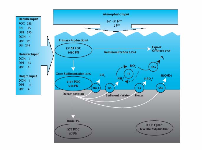
Figure 3.1
Nutrient budget for the North-Western Shelf of the Black Sea during the mid-1990s
(Mee, 2005, Mee et al, 2005, based on Friedrich et al, 2002)
i
All fluxes, except for measured river inputs, are calculated for a 50,000 km2 shelf area.
Data marked with # are taken from model calculations in Gregoire & Friedrich (2004) and
Gregoire & Lacroix (2003). Danube input represents the average input of 1991-1995
(Cociasu et al, 1996) except for POC and PN (Reschke et al, 2002). Dniester and Dnipro
inputs were taken from Topping et al (1999). Literature data on atmospheric inputs
reflect high uncertainties; values here are from Sofief et al (1994).
3.2.2 Secchi
depth
No Secchi depth data were available for the current assessment.
3.2.3 Turbidity
In essence, Secchi depth and turbidity are different measuring techniques for monitoring the same
parameter (light penetration through the water column). No turbidity data were available for the current
assessment.
3.2.4 Chlorophyll-a
Chlorophyll-a has long been used as an indicator of trophic status of fresh and marine waters, but
caution needs to be applied in the comparative analysis of results from different waterbodies or different
areas of large waterbodies, such as the Black Sea, since spatial difference may be high. Probably the
best example of this variability is from freshwater lakes, where for any given (limiting) nutrient
concentration, 95% confidence limits for long-term average chlorophyll-a results are an order of
magnitude apart (OECD 1982).
Chlorophyll-a is the only pigment present in all photosynthetic algae and higher plants, and is used as a
surrogate of phytoplankton biomass/standing crop when measured spectrophotometrically. Very few
data were available on chlorophyll-a measurements, and certainly not enough to make an assessment of
7
the trophic status of the North-Western Shelf in comparison to other areas of the Black Sea. However, a
considerable amount of remote sensing chlorophyll data has been collated and processed for the Black
Sea. It is these results which are discussed below.
Satellite data does not only include chlorophyll-a, however, it also records other types of chlorophylls
and chlorophyll-like substances. A major problem with the use of satellite imagery is, therefore ground-
truthing of the satellite data, Remote sensing chlorophyll-a data are usually calibrated/validated against
in-situ chlorophyll-a, but as the ratio of chlorophyll-a to other types of chlorophyll and chlorophyll-like
substances varies from between phytoplankton taxa, at any one time, satellite data provide only an
estimate of chlorophyll-a concentrations. The remote sensing chlorophyll maps of the Black Sea
presented in this report (e.g. Appendix B, Fig. B.12) show higher concentrations in the Sea of Azov, and
along the Bulgarian/Romanian/West Ukrainian coast, where the impact of the Danube would be
greatest. Remote sensing data records chlorophyll levels only in the very surface of waterbodies,
whereas laboratory-analysed chlorophyll-a levels can be measured for any depth from which water is
sampled.
Elevated chlorophyll levels in the Sea of Azov have been explained in terms of the shallow nature of the
water. While the reasons underlying this explanation remain unclear, they could also explain (partly at
least) the elevated levels in transitional waters of the Danube. Possible reasons for these elevated levels
are:
Ę Carry-over of freshwater phytoplankton into the Black Sea.
Ę Greater mixing of waters, resulting in increased resuspension of benthic material (including
detrital chlorophyll-like substances).
Ę Possible increases in phytoplankton growth rates (primary productivity) due to increased nutrient
concentrations. However, phytoplankton growth is not limited at nutrient concentrations greater
than 10 Ąg/l PO4-P in the presence of 100 Ąg/l dissolved inorganic nitrogen. It is paradoxical that
above these levels of nutrient concentration, although the rate of growth of phytoplankton does
not increase substantially, the standing crop of phytoplankton (and therefore chlorophyll-a) can
increase dramatically.
Ę The shallower the water, the more light that is available to drive planktonic photosynthesis.
Thus, the greater the primary productivity in shallow waters and the greater chance of increased
chlorophyll levels occurring.
3.2.5 Aquatic
vegetation
Two indicator species have been selected for use in the Black Sea: Cystoseira barbata (a brown
seaweed) and Zostera marina (a macrophytic sea grass). No data were available on the distribution of
these species within the Black Sea, but their presence/absence will be mandatory BSIMAP mandatory
parameters for monitoring during 2006-2011.
However, a methodology using rocky shore macroalgae morpho-functional indices to monitor trophic
status has been developed and tested at seven transects in the Sea (Appendix B, Section B.4).
The results of this assessment demonstrate a higher trophic status of rocky shores close to the Danube
delta than those further away, but concerns are raised that this methodology is more prone to local
influences (e.g. relatively small local discharges) than offshore biological methodologies (e.g.
zoobenthos assessments) when investigating the impact of the Danube.
3.2.6
Dissolved oxygen content
During the period 1990-1995, there was minor variability in dissolved oxygen levels in Romanian
coastal waters, with annual mean levels of 315-345 ĄM/l (Appendix B, Table B.3). These data suggest
8
that hypoxia was not a problem during this period, but hypoxia only needs to occur for a very short
period of time for ecological damage to occur.
From the early 1970s through the 1980s, tens of thousands of km2 of the Western Black Sea were under
hypoxic conditions (depleted oxygen). Oxygen levels increased throughout the 1990s, evidence of
which is presented in Section B.6.2 (Fig. B.20) with regard to mussel community age class distributions.
Clearly, the mussel beds have recovered to a large extent, particularly in the North of the North-Western
Shelf.
Further evidence of the onset of the increasing degradation of the North-Western Shelf waters
throughout the 1970s and early 1980s is shown in Fig. 3.2. The dramatic autumnal recovery in oxygen
status during the mid-1990s and early 2000s is illustrated in the lower half of the same figure.
Figure 3.2
Area of oxygen depletion (1974, 1978 and 1983) and percentage oxygen saturation
levels (1996, 1999 and 2003) in the North-Western Shelf of the Black Sea (Kroiss
2004)
2
3
1
200 m
Danube
Danube
Danube
45.0
120
1
90
60
40
100
140
80
50
120
100
44.6
30
100
90
80
80
40
5
0
7 6 0
0
0
100
1
70
0
44 .2
60
120
80
80
50
6
0
60
43.8
September 1996
September 1999
September 2003
29.0
30.0
29.0
30.0
29.0
30.0
3.2.7 Phytoplankton
Because of sampling and analytical methodology differences, data from Bulgaria, Romania and Ukraine
have not been comparable. However, at a recent workshop in Odessa (15-19August 2005) a first Black
Sea Regional phytoplankton intercalibration exercise was undertaken to facilitate comparison of
historical data, and agreement was reached over the use of standardised sampling/processing equipment.
No formalised lists of key taxa or other phytoplankton trophic status metrics have yet been made, but
these are expected as a reported output of the Odessa workshop.
Data are presented in Appendix B (Section B.5) for phytoplankton populations off the coast of Romania,
which show a marked change coinciding with the temporary return of eutrophic conditions in 2001.
However, the same data also cast doubt on the use of what has been considered one of the most robust
9
phytoplankton trophic status indicators (the diatoms:dinoflagellates ratio), when used in terms of cell
numbers. No data on phytoplankton biomass were available to compare results.
3.2.8 Zooplankton
No data were available on zooplankton biomass, percentage of key groups or No of Noctiluca. Because
of sampling and analytical methodology differences, historical data from Bulgaria, Romania and
Ukraine have not been comparable. However, at a recent workshop in Odessa (15-19 August 2005) a
first Black Sea Regional zooplankton intercalibration exercise was undertaken to facilitate comparison
of historical data, and agreement was reached over the use of standardised sampling/processing
equipment. No formalised lists of key taxa or other zooplankton trophic status metrics have yet been
made, but these are expected as a reported output of the Odessa workshop.
3.2.9 Macrozoobenthos
(biomass,
percentage of key groups)
Macrozoobenthos populations of the North Western Shelf are discussed in detail in Appendix B, Section
B.6. The Danube Delta region of the Shelf shows clear signs of impact from the Danube itself, although
the zoobenthic population is not as heavily impacted there as it is closer to Odessa, where other sources
of contamination and disturbance are likely to be the predominant causative factors. Other areas of the
North-Western Shelf are less heavily impacted.
While there are still obvious signs of the impact of the Danube, the situation has improved substantially
from that in the mid-late 1990s (Appendix B, Section B.6), but a reversal of the status of the zoobenthos
ecosystem to that observed in the 1980s and early 1990s is still possible. For example, year 2001 was a
dry year, causing reduced mixing of waters and resulting in extensive hypoxia, leading to the death of
benthic organisms. In Fig. B.20, for example, recruitment of young mussels in 2001 (1+ for year 2003)
was very low in marine areas south of the Danube Delta, but much improved in more northerly waters.
3.2.10 Pollutants
Sediment contamination with organic and inorganic contaminants is discussed in detail in Appendix B,
Section B.7. Overall, results indicate an impact of the Danube on coastal sediments of the North
Western Shelf, particularly with regard to heavy metals, albeit that any increases in sediment
contamination levels are relatively small when considering the catchment area of the Danube compared
to the catchment area of coastal land which drains directly into the North Western Shelf.
Levels of contamination at individual sites will reflect land export of contaminants as a result of
contaminant production/use in coastal areas, direct discharges to the marine environment, illegal waste
dumping at sea and atmospheric deposition, as well as river inputs. While surface sediment samples
were used for the vast majority of the analyses presented, there is also the risk of a historical `shadow'
reflecting sediment contamination. This is primarily due to bioturbation Ł mixing of marine sediments
by burrowing animals - so older, deeper and possibly more contaminated sediments (reflecting levels
occurring before the Danube clean-up programme of the 1990s and early 2000s) may become
incorporated into surface sediments.
For a number of chlorinated pesticides (dieldrin, lindane, opp DDD, opp DDT, pp'DDD, pp'DDT,
DDMU, op'DDE, pp'DDE and HCHa) the highest concentrations were found in Ukrainian sediment,
with concentrations diminishing in a southerly direction. For two of these contaminants (dieldrin and
op'DDE), however, increased concentrations were again recorded in Bulgarian sediments. Elevated
levels of HCB, HCH, lindane, heptachlor, aldrin and endosulfan were also detected at Bulgarian sites.
For three pesticides (cis- and trans-chlordane and a-HCH), maximum levels were associated with the
Sulina branch of the Danube, although for a-HCH, comparable levels were detected at a number of other
sites.
10
The massive level of DDT contamination recorded at one Ukrainian site is considered much more likely
to reflect illegal discharges/dumping than land run-off.
PCB concentrations were highest at more northerly sites of the North-Western Shelf. Maximum
concentrations of ten PCBs (aroclor 1260, PCBs 149, 153, 170, 174, 177, 180, 183, 187 and 194) were
associated with Danube River input via the Sulina Channel. For a further twelve PCBs (aroclor 1254,
PCBs 44, 49, 52, 87, 101, 105, 110, 118, 128, 138 and 201) maximum concentrations were recorded in
Ukrainian sediment, levels which could also reflect inputs from the Dneister and Dnipro rivers.
Sediment concentrations of all PCBs except one (PCB 201) were low in north Bulgarian sediment, but
for most PCBs greater contamination was detected in southerly Bulgarian sediments.
For eight metals, highest sediment concentrations are associated with inputs from the Sulina Branch of
the Danube Delta, albeit that elevated levels of contamination of some metals (cobalt, nickel copper and
aluminium) were also noted in samples from off the coast of southern Bulgaria. A sampling site off the
coast of Ukraine also had elevated levels of arsenic. However, as stated for organic contaminants, the
Ukrainian result is also likely to reflect greater influence of inputs from the Dnipro and Dneister rivers.
11
12
4.
THE BLACK SEA REGIONAL INTEGRATED
MONITORING AND ASSESSMENT PROGRAMME
(BSIMAP)
4.1 Background
The underlying principles of the Convention on Protection of the Black Sea against Pollution imply a
holistic approach to monitoring and assessment of the Black Sea ecosystem. These principles have been
considered in the development of the Black Sea Integrated Monitoring and Assessment Programme
(BSIMAP), which seeks to maximize the use of historical data from previously established monitoring
sites for trend analysis, supported by new additional sites to improve the assessment of the current
chemical/ecological status of the Black Sea. The main purpose of the BSIMAP is therefore to provide
data for `state of the environment' reporting, but the sites, parameters and monitoring frequencies also
reflect data requirements for compliance with other national and international legislation and
agreements. The same data should also be suitable for undertaking broad-scale `impact assessment'
investigations of major pollutant and water sources, such as assessing the impact of major rivers (in this
case the Danube, the largest river feeding the Black Sea). However, for impact assessments to be
undertaken, unimpacted baseline conditions need to be established.
4.2
BSIMAP aims and purposes
A consensus was reached by the BSC institutional network (including its Pollution and Monitoring
Advisory Group) that the BSIMAP should:
1. Build on established national monitoring programmes.
2. Be compatible with underlying WFD principles.
3. Utilise standardised, sampling, storage, analytical techniques, assessment methodologies and
reporting formats. [Reporting formats have been specified, but are sometimes not followed.
Standardised manuals for phytoplankton, zooplankton and zoobenthos are currently being
updated and a series of workshops were held during summer/autumn 2005 to promote
harmonization of techniques and train workers from all coastal countries. Standardised
procedures for nutrient analysis and chlorophyll-a have also been produced.]
4. Include agreed quality assurance/quality control procedures. [These have not yet been fully
established. However, a draft mission report from December 2002 (now somewhat out of date),
prepared by Dr Stephen de Mora and Dr Oksana Tarasova is included as Appendix G, describing
the infrastructure, equipment and staff available (primarily for chemical analysis) in those
organisations responsible for Black Sea monitoring in five of the six riparian countries (Georgia
is excluded). Limits of detection and accuracy and precision targets are not specified for any
parameters.]
A first regional quality assurance intercomparison exercise was undertaken in 2004 for metals,
nutrients, chlorinated pesticides and petroleum hydrocarbons. Seven laboratories from five
countries participated (no Turkish laboratories took part in the exercise), albeit with different
laboratories participating for different groups of chemicals The results of this exercise remain
confidential, but as may be expected from the first exercise of this type, the results suggest that
there is a considerable amount of work required by the participating laboratories. During 2005,
the Black Sea Commission provided the funds for all countries to participate in the IAEA-MEL
Quasimeme chemical quality assurance exercise. Additional quality assurance exercises are
13
planned for 2005/2006 on nutrients in seawater, organic contaminants in sediment and heavy
metals in sediment as part of the BSERP.
Preliminary results from plankton intercalibration exercise undertaken during August/September
2005 show a major variability in results obtained by individual laboratories, differences which in
large part are probably due to the alternative methodologies and equipment used by individual
countries. The workshop on macrozoobenthos, included an intercomparison exercise (again with
some important inter-laboratory differences being reported), albeit with full agreement having
been reached on a standardised methodology and equipment for use by all six countries.]
5. Be affordable. [The economies of the six countries are all suffering to various extents, with that
of Georgia being most depressed. With environmental matters being low on the political agenda,
funding for environmental monitoring tends to receive scant political support, so while a
comprehensive list of parameters and high monitoring frequencies can be supported technically,
from a pragmatic viewpoint, a smaller list of monitoring sites, less expensive parameters and less
frequent sampling/monitoring is more likely to achieve governmental funding. Clearly, those
countries aiming for EU accession in the near future (Romania and Bulgaria; Turkey at a later
date) will need to comply with the monitoring requirements of EU Directives. In general terms,
organic compounds are more expensive to analyse for than inorganic compounds, and not all
countries have the equipment or technical ability to analyse for them. However, not all countries
have the capacity/ability to analyse for some inorganics, e.g. mercury.]
The Black Sea Commission and its advisory bodies/institutional framework believes that to achieve
further harmonisation, common environmental quality criteria/objectives should be established and the
Black Sea Information System further developed to facilitate regional State of the Environment
reporting.
4.3 Reference/baseline
conditions
The establishment of baseline (reference) conditions is at the heart of the EU Water Framework
Directive (WFD), since all biological monitoring results should be presented in the form of
environmental quality indices (EQIs), i.e.:
Result at monitoring site
EQI = Result at reference site
Reference conditions for impacted sites can be established using three main approaches:
Ę Status at quasi-pristine (but otherwise comparable) site
Ę Expert judgment
Ę Modeling
However, the reality is that the first of these three methods is the most practical and robust, particularly
when considering ecological monitoring. The reasons for choosing some individual monitoring site
locations remain unclear, although as already indicated, there is a historical justification for many of
these sites to enable trend analysis using historical data.
4.4 BSIMAP
proposed
spatial
coverage
Perhaps the most obvious aspect of the BSIMAP is that it is restricted to the Black Sea Ł there are no
monitoring sites in the Sea of Azov. While it is very obviously a transboundary waterbody, both the
Ukrainian and Russian governments consider it to be outside of the scope of BSIMAP, despite its
influence on the Black Sea. However, some protocols of the Black Sea Commission also cover the Sea
of Azov. These include the Black Sea Biodiversity and Landscape Conservation Protocol and the draft
14
revised Protocol for the Protection of the Black Sea against Pollution from Land-Based Sources and
Activities.
Article I of the Convention (on the Protection of the Black Sea against Pollution) defines the area of
application as the Black Sea proper, with the southern limit constituted by the line joining Capes
Kelagra and Dalyan. It also states that the Black Sea shall include the territorial sea and exclusive
economic zone of each Contracting Party in the Black Sea. However, any protocol to the Convention
may include areas outside of the Black Sea `proper' for the purposes of that protocol. The Black Sea
`proper' is thus interpreted as excluding the Sea of Azov.
In 2005, the Turkish government funded monitoring at an additional 63 sites (Table 4.1), with many of
these sites being relatively unimpacted. Thus, over half of the current BSIMAP sites are now along the
Turkish coast, greatly improving the spatial coverage of the integrated programme (see Fig. 4.1, with
coordinates shown in Appendix F), albeit with the Ukrainian and Russian coasts still remaining only
sparsely covered. Improved spatial coverage of BSIMAP remains an aim of the Black Sea Commission
Permanent Secretariat. It is hoped to increase the number of Georgian and Russian monitoring sites in
future years.
Table 4.1
Number of national monitoring sites included in the BSIMAP, with an indication of
spatial coverage
Territorial waters
Pollution Sampling sites
Length of coast, Average distance
of
hot spots
km
(km) represented
per sampling site
Bulgaria 9
5
300 60
Georgia 6
5
310 62
Romania 5
21
225
17
Russian Federation 4
5
475
95
Turkey
10
3 (66 from
1400
466 (21 from
2005)
2005)
Ukraine 9
14
1628 116
4.5 BSIMAP
parameters
A list of compulsory and recommended (optional) parameters has been specified by the BSC Permanent
Secretariat. The paucity of national funding for environmental monitoring means that only mandatory
parameters are considered in this report, since optional parameters tend to be monitored by few (if any)
countries. Mandatory parameters are shown in Appendix H.
This list of compulsory parameters does not fully tie-up with the list of indicators agreed by the JTWG,
and detail is sometimes omitted from the recommendations. The recommendations for monitoring in
2005 include phytoplankton as the only mandatory biological parameter.
For nitrogenous nutrients, data are requested for ammonia, nitrite and nitrate, but for reporting purposes
it would preferable to add these parameters together to give dissolved inorganic nitrogen (DIN), an
accepted surrogate of bioavailable nitrogen, albeit composed overwhelmingly of nitrate. Total nitrogen
and total phosphorus are also requested as part of the BSIMAP but, to date, few countries have
monitored theses as standard parameters.
15
Figure 4.1
BSIMAP proposed monitoring sites, 2005
Ukraine
Russian Federation
Romania
Bulgaria
Georgia
Turkey
16
The list of 2005 compulsory parameters does not adequately tie-up with the list of indicators agreed by
the Black Sea-Danube JTWG (Section 2), e.g. phytoplankton as the only mandatory biological
parameter (Appendix H, Table H.1). However, the revised list of compulsory parameters for 2006-2011
Appendix H, Table H.2), proposed at a recent PMA Advisory Group meeting, much more closely
matches the agreed list of indicators, but detail is sometimes missing from both the agreed list of
indicators and the specified reporting parameters of the Black Sea coastal countries. For example, no
decisions appear to have been made on the format for reporting macrozoobenthos data Ł although
biomass and percentage of key groups has been agreed on as the indicator, should these key groups be
taxonomic or functional feeding groups (Appendix B, Section B.6). Alternatively, should a biotic index
be used (Section 6.9)? This also poses very large questions for data collation/storage as part of the Black
Sea Information System (BSIS): should raw data be quested by the Commission or processed data?
Clearly raw data would be of benefit for future development work on indicators. In addition there is still
a need to reach agreement on standard taxonomic lists for use by all countries; at present different
countries are still calling some taxa by different names.
Monitoring for a limited number of toxic heavy metals (cadmium, copper, mercury and lead) is
mandatory within the BSIMAP, which appears appropriate given the limited funding available.
However, the addition of other heavy metals should require only a marginal increase in expenditure and
is likely to be beneficial for future impact assessment studies. No guidance is presented on whether
total or dissolved heavy metals should be monitored Ł this is an important consideration which should
be addressed in terms of loading to the Sea, bioaccumulation and toxicity to marine biota.
4.6
BSIMAP proposed monitoring frequencies
Up until 2005, the BSIMAP specified the same monitoring frequency for all compulsory parameters in
all countries (Appendix H). For most of the compulsory parameters (phytoplankton, nutrients, petroleum
hydrocarbons, salinity, oxygen balance parameters, suspended solids and physico-chemical parameters)
this frequency is set at 4 times per year.
For fish catch statistics annual reporting is required, which again appears pragmatic, given how the data
are reported nationally.
For the four heavy metals, a monitoring frequency of only once per year is specified by the Black Sea
Commission Permanent Secretariat. This appears to be an extremely low monitoring frequency for
analysis of either trends or step changes, and is likely to result in only very large changes being detected
at a statistically significant level. However, at a recent meeting of the PMA Advisory Group, during a
discussion on whether monitoring of heavy metals in the water column should be mandatory (as
opposed to monitoring of sediment contamination), it was stated that the purpose of monitoring the
water column was only to define `background levels' throughout the Sea.
While the Commission specifies a minimum monitoring frequency of 4 times per year for most of the
compulsory parameters, Bulgaria aims to samples seven times a year, and will continue to do so, while
at the 63 new (2005 onwards) Turkish sites, monitoring will only be undertaken twice a year.
4.7
Recent years BSIMAP reporting
Appendix I shows the maximum number of results reported to the Black Sea Commission for samples
collected during the years 2001 (Table I.1) and 2003 (Table I.2) for each of the BSIMAP sites. Sites 51
to 113 (see Appendix F) are excluded from these tables, since formal monitoring only began at those
sites during 2005. For Tables I.1 and I.2 results are grouped into the following categories:
17
Ę Oxygen balance parameters (including BOD5, dissolved O2 [% saturation] and dissolved O2
[mg/l])
Ę Nutrients (including ammonia, nitrite, nitrate, silicate and ortho-phosphate Ł neither total P nor
total N are monitored by any laboratory)
Ę Heavy metals (including cadmium, copper, mercury and lead)
Ę Organic pollutants (petroleum hydrocarbons)
Ę Other water column physico-chemical parameters (including temperature, pH, salinity, total
suspended solids and Secchi depth)
Ę Chlorophyll-a
The information in Appendix I therefore represents a rather optimistic view of historical monitoring. For
example, if BOD5 had only been reported on three occasions during 2001, but dissolved oxygen (%
saturation and mg/l had both been reported on 10 occasions during that year, then the oxygen balance
parameters group would be shown as having been monitored on 10 occasions (250% of the
recommended monitoring frequency). The tables show enormous variability in the number of reported
data for individual sites and in the types of parameters which were monitored, making the BSIMAP
appear rather uncoordinated.
18
5.
CONSIDERATIONS FOR IMPROVING THE COLLECTION
AND INTERPRETATION OF BLACK SEA MONITORING
DATA
5.1 Funding
and
equipment
Perhaps the most obvious statement to make is that there is little use in defining or agreeing to a
monitoring programme if insufficient funds are made available to measure the minimum (mandatory)
monitoring parameters. This funding needs to cover transportation costs (including provision of a
boat/ship), monitoring and analytical equipment costs, including consumables, as well as staff costs.
5.2
Relevant and proposed legislation
The most relevant international policies and agreements in terms of monitoring the Black Sea are
considered to be the Strategic Action Plan for the rehabilitation and protection of the Black Sea, the
Water Framework Directive and the proposed Marine Framework Directive.
5.2.1
Strategic Action Plan for the rehabilitation and protection of the Black Sea
Article 54 of the Black Sea Strategic Action Plan (BSSAP) states that "A Black Sea Monitoring System,
based upon biological effects measurements and measurements of key contaminants will be established
in compliance with the Bucharest Convention. It will consist of the integration of obligatory monitoring
programmes, to be included in the National Strategic Action Plans, and an independent quality
assurance system. It is advised that the Istanbul Commission develop such a quality assurance system
through its advisory group on Pollution monitoring and assessment by 1998." The Black Sea SAP will
shortly be updated for presentation to the Black Sea Commission and the six national governments
5.2.2
Existing European Union directives
Bulgaria and Romania are expected to join the European Union in 2007. Turkey is a candidate country
with whom accession negotiations have not yet started. Once these countries have joined the EU they
will have to implement the EU legislation relating to marine waters.
The most significant EU policy relating to the water environment is the Water Framework Directive.
The Water Framework Directive covers all waters, including inland waters (surface water and
groundwater) and transitional and coastal waters up to one sea mile (in terms of monitoring ecological
status and for the chemical status also territorial waters which may extend up to 12 sea miles) from the
territorial baseline of a Member State, independent of the size and the characteristics.
Member States have to characterise their waters in terms of numbers and types of water bodies, and
identify the pressures upon them. A surface water body is defined as a discrete and significant element
of surface water such as a transitional water or a stretch of coastal water. The main purpose of
identifying "water bodies" is to enable status to be accurately described and compared to environmental
objectives. Physical features (geographical or hydromorphological) should be used to identify discrete
elements of surface water. A water body should not contain significant elements of different status and
must be capable of being assigned to a single ecological status class with sufficient confidence and
precision through the Directive's monitoring programmes.
To that end, Member States have to implement monitoring programmes that enable the classification of
surface water bodies into one of five classes. Monitoring is termed surveillance, operational or
investigative each with defined objectives. Operational monitoring is to be undertaken in water bodies
thought to be at risk of failing environmental quality objectives and will focus monitoring on those
determinands most relevant to the pressures creating the risk. Surveillance monitoring should include
19
sufficient water bodies to provide an assessment of the overall surface water status within each
catchment and sub-catchment of the river basin district: to achieve this water bodies not at risk (i.e. high
and good status) and those at risk will have to be monitored. Member States will also have to determine
how many monitoring stations are required in each water body (or groups of water bodies) to determine
its status.
Bulgaria and Romania have identified and characterised their water bodies as required by Article 5 of
the Water Framework Directive: two coastal water bodies and types were identified along the 300 km of
Bulgaria's, and three water bodies and two types identified along the 225 km and Black Sea coastlines
(Member States are only required to identify water bodies in coastal waters, not territorial waters). For
comparison 556 coastal waterbodies have been identified in the UK along 5167 km of coastline, giving
approximately one waterbody per 9.3 km. In Bulgaria and Romania there is an average of one water
body per 150 km and 75 km of coastline, respectively.
The European Commission is also developing a Daughter Directive to the Water Framework Directive
under Article 16 on environmental quality standards and emission controls for Priority Substances. At
the present time environmental quality standards for the concentration of the substances in water
(including coastal waters) will be established, but not for concentrations in biota or sediment. The
Daughter Directive will re-iterate the need for these substances to be monitored not only in water for
determining chemical status and checking compliance with the EQSs, but also for their presence in
sediment and biota to demonstrate compliance with the "no-deterioration" objective of the Water
Framework Directive (Article 4(1)(i).
Monitoring of surface freshwaters, estuarine, coastal and marine waters is also required for the Nitrates
Directives where marine waters are referred to as those in "exclusive economic zones". The geographic
extent of marine waters included in the requirements of the Urban Waste Water Treatment Directive is
not clear: Annex II, (criteria for the identification of sensitive and less sensitive areas) includes estuaries
and coastal waters in terms of sensitive areas, whereas marine water bodies are included in the criteria
for less sensitive areas. Coastal waters are defined as "waters outside the low-water line or the outer
limit of an estuary". The European Commission has developed informal guidance on monitoring
required for the Nitrate's Directive which includes water quality determinands such as nitrate but also
relevant biological determinands such as phytoplankton, aquatic vegetation, benthic invertebrates and
fish.
The European Commission is also developing guidance on eutrophication for the Water Framework
Directive. It compares how eutrophication is understood, defined and assessed in EC Directives,
policies, guidance and research, and proposes a new conceptual framework for eutrophication
assessment across all water categories and policies. The guidance includes a chapter on monitoring with
the aim of integrating the monitoring requirements stemming from the various obligations dealing with
eutrophication.
5.2.3
Proposed Marine Framework Directive
The proposed Marine Framework Directive (arising from the Commission's Marine Strategy) would be
applicable to all European marine waters under the sovereignty or jurisdiction of the Member States. It
would, therefore, cover marine waters within a country's exclusive economic zone (up to 200 nautical
miles from the baseline from which the breadth of territorial waters are measured). The strategy is also
directed at non-EU countries bordering these areas (presumably including those Black Sea countries that
are not EU candidate countries) and at the relevant international organisations in which countries
cooperate (e.g. the Black Sea Commission). The objective of the Directive would be to protect, conserve
and improve the quality of the marine environment in these marine waters through the achievement of
good environmental status within a defined time period. The directive will define/establish ecosystem-
20
based marine regions as the implementation unit. The latter will be defined on the basis of their
hydrological, oceanographic and bio-geographic features. Monitoring and assessment programmes will
have to be developed for each marine region taking into account existing monitoring and assessment
programmes. Monitoring would also be required offshore of territorial waters within economic zones,
the delineation of which has not yet been completed by all Black Sea countries. It is, therefore, likely
that the geographical extent of monitoring of the Black Sea will have to be increased by at least some of
the Black Sea countries.
5.3
Spatial and depth coverage of monitoring stations
Table 4.1 and Appendix F summarise the numbers of stations per country and the average distance
represented per sampling site. If the spatial coverage of stations could be increased then new stations
should not only be located to detect potential impacts from identified sources (hot spots) such as point
source discharges or diffuse inputs via rivers, but also at points further away where impacts are expected
to be less. In particular reference sites (see below) should be established against which values of
determinands measured at the impacted sites could be compared. The approach used in Romania seems
an appropriate one if resources are limited, where stations have been established seaward along a line
perpendicular to the coast where the main sources of pollution appear to be. Of course stations further
offshore may also be impacted by pollutants carried by the prevailing currents from other parts of the
Black Sea. Similarly, the zone of influence of river inputs and major discharges should also be covered
by monitoring.
The selection of stations (and determinands to be monitored) would also be facilitated by the approach
adopted for the Water Framework Directive, that is transitional and coastal waters are characterised in
terms of the types and numbers of water bodies and then the pressures potentially impacting them
identified. The identification of pressures includes those arising from point sources along the coast and
offshore, diffuse sources such as pollution from shipping and the flows from the larger rivers. This is the
process that Romania and Bulgaria have started as candidate EU countries and which Turkey will start
at some point in its EU entry negotiations.
The typifying of water bodies helps the comparison of like-with-like when it comes to comparing
monitoring results and assessing state from different parts of the same country and across the Black Sea
as a whole. For example, comparing the biological community attributes and metrics (such as diversity)
from relatively low salinity and shallow parts of the Black Sea with relatively high salinity deep parts of
the Black Sea may not be valid and lead to the wrong conclusions about their relative quality. The
division of coastal waters in terms of types and potential status could help obtain (through surveillance
monitoring) a representative view of quality along the coast rather than just of the worse quality areas.
The physical factors that could be considered in determining whether stations are within water bodies or
areas of similar and comparable types would include depth of water, salinity, degrees of exposure and
sea bed characteristics (i.e. sedimentary or rocky). The Water Framework Directive working group on
intercalibration identified three depths for the identification of comparable types for intercalibration:
shallow with a depth of less than 30 m, of intermediate depth 30 to 50 m and deep greater than 50 m.
For example, in the Black Sea a `natural' decrease in macrozoobenthic community diversity is observed
in the deeper waters of the North-Western Shelf reflecting the greater environmental stress at these
depths. In terms of salinity, the least saline parts of the Black Sea are in the North-Western Shelf in
relation to the main river inputs. Differences in salinity should be taken into account when monitoring
for any biological determinands as aquatic communities will vary in relation to salinity. Nitrate
concentrations will also vary in relation to salinity particularly as the rivers are significant sources of
nutrients to the Black Sea. Allowing or normalising for salinity will improve the robustness of trend
analysis of nitrate concentrations at stations where salinity varies significantly between sampling
occasions.
21
In terms of depth the sampling for some water quality determinands such as nutrients and chlorophyll
should take into account the potential vertical stratification of the water column (e.g. presence of a
pycnocline) and the varying depths of maximum phytoplankton biomass. For example samples for
chlorophyll would ideally be taken throughout the euphotic zone at regular intervals or by taking
continuous measurements with a fluorometer. Once a few seasons/years of data have been obtained the
results could be statistically assessed to see if there was any opportunity to reduce the number of
samples without losing any information (i.e. where maximum chlorophyll concentrations are occurring).
As an example, for the Baltic Sea the standard sampling depths for chlorophyll-a are 1 m, 5 m, 10 m, 15
m and 20 m. Samples integrated over 1 to 10 m are also acceptable.
One of key criteria of the present BSIMAP is the affordability of monitoring in each of the countries. It
is quite clear that the present monitoring in some of the countries is not adequate to obtain an overview
of the state of coastal waters of the Black Sea (and also maybe not for the assessment of all hot spots).
As the largest proportion of the total cost of monitoring probably is generally with undertaking sampling
(ships, personnel etc.) cruises (compared to the cost of sample analysis) then it might be the better
option to undertake sampling at more stations and at an increased number of depths over the water
column for water quality samples, rather than increasing the monitoring frequency. In addition, more
monitoring stations in the open, offshore waters of the Back Sea (particularly in the North-Western
Shelf area and in the deeper central area) would enable a more complete spatial assessment of water
quality/ecological status to be made.
No guidance is currently offered to countries on the depth at which water should be sampled. Nutrient
and chlorophyll-a concentrations (in particular) will differ with depth, particularly when a summer
thermocline is established. The existence of a very obvious halocline in the Black Sea will also result in
different concentrations above and below the pycnocline.
5.4
Reference site selection
Stations should ideally be selected in water bodies/areas that represent the least impacted parts of the
Black Sea. They should also be selected where possible in a range of types of water bodies/areas to
account for any differences in the monitored determinands between stations that arise from natural
factors rather than from differences in anthropogenic pressures when comparing monitoring results.
The Water Framework Directive requires Member States to establish type-specific reference conditions
which "equate to the values of the biological quality elements for the surface water body reflect those
normally associated with that type under undisturbed conditions, and show no, or only very minor,
evidence of distortion." These conditions would be equivalent to high ecological status. Not many
Member States will be able to identify and monitor stations and water bodies that are at high ecological
status: this may also be the case in the Black Sea as it is effectively isolated from the World Ocean and
is very vulnerable to pressures from land-based human sources. However Member States are able to use
temporal reference conditions reconstructed from historical records Ł early 20th century.
If reference conditions are not present in the Black Sea and temporal reference conditions cannot be
established, then the least impacted stations could be used for comparisons of relative quality and state.
In either case a number of reference stations should be selected to be representative of all the different
water types/areas in the Black Sea. In addition, reference stations/conditions can be "shared" by
countries in the case where they do not exist in the coastal waters of one country but do so in another.
Thus the monitoring results obtained (assuming the same methods and metrics are used) from the
reference station in one country, could be used as a baseline for comparison of the results from the
impacted station in another country. However, to make the resultant comparison and assessment of
results/status valid, the water bodies/areas must be of the same type.
22
Reference sites/conditions for individual impacted sites are not specified on the BSC website. The
proposed inclusion of macrozoobenthos as a mandatory monitoring parameter opens a very large issue
in terms of the BSIMAP site selection, since many of the current BSIMAP sites appear to have been
selected primarily for water column chemistry/hydrology monitoring. Sediment particle size can make
an enormous difference to what taxa live in/on the sediment and the level of contaminants adsorbed onto
that sediment. The identification of sediment reference sites therefore remains open. While different
sites could be selected for monitoring water column and sediment parameters, the underlying principles
of an `integrated' monitoring programme strongly suggest that the same (vertical) sites should be
selected for monitoring all parameters/metrics.
5.5 River
inflows
Rivers have been identified as important sources of pollutants into the Black Sea with the Danube,
Dnipro and Dniester being the biggest rivers in terms of flow discharging into the North-Western Shelf
area of the Black Sea. There appears to be two main reasons for monitoring the main rivers discharging
into the Black Sea, to determine the riverine loads entering the sea and to assess the impact of the
pollutants in the river water on the Black Sea ecosystem. Black Sea countries undertake some
monitoring of riverine loads but as the Black Sea Commission states the data are not always reported in
a harmonised way. It would be of value if the quantification of riverine loads (as well as other pollution
sources) could be standardised and harmonised to obtain a more accurate assessment of loads entering
the Black Sea. Good examples of how this has been undertaken by other Marine Conventions are the
RID and PLC guidelines produced by the OSPAR and HELCOM Commissions, respectively. The
Danube has a very well established river monitoring network (TNMN) with a load assessment
programme that started in 2000 with countries agreeing to use a standard operational procedure for the
measurement and calculation of riverine loads from the Danube into the Black Sea. Procedures giving
comparable results should be adopted for the assessment of loads at the most downstream points in other
major rivers discharging into the Black Sea.
A number of surveys have been undertaken of the North-Western Shelf to assess the impact of river
discharges and other pollution sources. Comments have also been made about the spatial coverage of
monitoring stations: more stations would be required in BSIMAP to more accurately quantify the impact
of major rivers. For example, 60 stations were sampled to assess status if the macrozoobenthic
communities into the North Western Shelf (Todorova et al, 2004). The potential importance of salinity
as a factor influencing water quality determinands and aquatic biological communities has also been
discussed earlier.
5.6
Seasonality and sampling frequency
In an ideal situation sampling would be undertaken at a frequency high enough to determine the inherent
variability of the monitored determinands in all the different water types/areas in the Black Sea. This
implies an initial high frequency of sampling, for example, at least monthly for some of the water
quality determinands such as nutrients and chlorophyll. An assessment can then be made as to the
optimum frequency to obtain an adequate level of confidence and precision in the information that is
required e.g. to detect maximum chlorophyll and nutrient concentrations or to assess average conditions
from year-to-year.
Annex V of the Water Framework Directive provides tabulated guidelines in terms of the minimum
monitoring frequencies for all the quality elements. The suggested minimum frequencies are applicable
to both surveillance and operational monitoring and are generally lower than currently applied in some
countries. More frequent monitoring will most likely be necessary in many cases to achieve a reliable
assessment of the status of the relevant quality element, but also less frequent monitoring is justified
when based on technical knowledge and expert judgment. The Black Sea Commission has considered
23
the Water Framework Directive requirements when proposing monitoring frequencies for the different
elements of the BSIMAP.
In terms of Marine Conventions, HELCOM defines frequent and highly frequent monitoring stations
(some high frequency stations are sampled up to 26 times/year or even more often) that have
recommended sampling frequencies higher than the minimums given by the Water Framework
Directive and Nitrates Directive. However a common theme between those Directives that require
monitoring of marine waters and other Marine Conventions that could be incorporated into BSIMAP is
the recognition that sampling should be targeted to specific times of year for some of the determinands
(e.g. nutrients in winter and chlorophyll during maximum chlorophyll production). There is also a
common theme in a number of European Directives and international agreements of ensuring that
monitoring results are fit for purpose and this implies that different frequencies would be required for
different quality elements, different water categories (transitional, coastal and open marine waters) and
different water bodies. As examples: Member States have to achieve acceptable levels of precision and
confidence in the monitoring results and subsequent assessments (Water Framework Directive);
Contracting Parties have to determine optimum sampling frequencies, for example, to confirm
maximum winter nutrient concentrations have been determined (OSPAR) or to detect changes in
concentrations over 10 years (MEDPOL).
The analysis of historical datasets on water quality indicates clear seasonality in relation to dissolved
oxygen, ammonium, nitrate and silicate concentrations. In these cases the detection of significant trends
in quality over time might be improved by aggregating data not only annually but also for specific
seasons such as winter for nitrate. Sampling for nitrate and other nutrients, however, should ideally be
undertaken throughout the year.
Benthos shows considerable numerical variability over a year due to larval recruitment and mortality.
The results of repeated surveys are more easily compared if they are carried out at the same time of year,
for example within +/- 3 weeks of an agreed date or the date of the first annual survey. For the North
Sea the best time to sample in order to avoid the largely ephemeral larval recruitment is the first six
months of the year. However, because of bad winter weather the sampling period April to June is
generally used. In the Baltic Sea sampling is undertaken in May or June in Finland and Sweden, and in
August in Latvia. OSPAR recommends sampling to be undertaken between June and September. The
recommended sampling period for BSIMAP is in April and then again in September/October: this is
consistent with approaches adopted in other seas.
5.7
Historical data availability for trend analysis
The data sets compiled and assessed for this report have provided some good quantitative information
on the state of, and trends, in the North-Western Shelf area. The historical data would also be useful in
determining the spatial and temporal variability of some of the monitored determinands: this would be
useful if additional monitoring stations and revised monitoring frequencies were to be considered for
BSIMAP. It would also be worth considering including some of the stations used in the various research
cruises in BSIMAP to maintain the already available time series.
5.8
Sources and types of current and historic pollutants
The impact of as many major pollution sources as possible should be monitored as far as is possible
under BSIMAP bearing in mind the affordability to do so in each of the countries. The cruise to screen
pollutants in sediments revealed some very interesting results in terms of the relatively high
contamination levels of some substances (some pesticides, some heavy metals, and PCB) found at a few
locations off the coasts of Bulgaria and Ukraine. The concentrations of some substances are in or above
the ranges used as Ecotoxicological Assessment Criteria (EAC) by OSPAR. EACs are defined as
concentration levels of a substance above which concern is indicated, and have been used by OSPAR to
24
identify possible areas of concern and to indicate which substances might be a target for priority action.
Whilst the applicability to the Black Sea of EACs developed for the NE Atlantic is not known, the
significance of the detected contamination should be further investigated and if possible the monitoring
of contaminants in sediment and biota should be considered for inclusion as mandatory elements in the
BSIMAP.
5.9 Pollution
impacts
One of the aims of monitoring is to determine the impact of pollution. In terms of the Water Framework
Directive this would be expected when pollutants were causing the degradation of ecological and
chemical status to be less than good. Ecological status is monitored and assessed in terms of defined
biological quality elements: these elements are included as either mandatory or optional elements of
BSIMAP. The results obtained from BSIMAP when compared to appropriate reference
levels/conditions would give a measure of impact. For example the assessment of macrozoobenthos in
the North-Western Shelf has detected pollution effects.
The European Commission is in the process of developing environmental quality standards for Priority
Substances: compliance with these standards will equate to the achievement of good chemical status. At
the present time, annual average and maximum allowable concentration standards for the water phase in
inland surface waters and other surface waters (presumably transitional and coastal waters) are being
proposed. There are no standards yet being proposed for the substances in sediment and biota. These
standards could be applied to BSIMAP monitoring results once they are available.
In addition, the use and possible adaptation to Black Sea conditions (if technically necessary) of the
Background/reference concentrations, and Ecotoxicological Assessment Criteria developed and used by
OSPAR for assessing the significance of monitoring undertaken in its Convention area could be used
(see also Section 5.8). In the longer term it may also be possible to use direct biological effects
measurements such as oyster embryo water bioassays and whole sediment bioassays with amphipods
and annelids: such measurements have been used in the OSPAR Convention area.
5.10
Data analysis and interpretation
The importance of robust statistical techniques for assessing spatial differences and temporal trends in
water quality data sets have been demonstrated by the analysis undertaken on historical datasets in
Appendix B.2. For example, significant seasonality was found in some of the nutrient data sets. Such
periodicity in data sets needs to be understood and accounted for if valid trend assessments are to be
undertaken. The targeting of monitoring to specific times of year and to specific types of water body
(e.g. in terms of depth and salinity) might also serve to reduce some of the inherent variably of the
measured determinands. There are well established, robust and accepted statistical methods for trend
analysis such as the Mann-Kendall Statistics used by the European Environment Agency to detect
significant trends in marine water quality datasets used in its indicators. It is expected that appropriate
statistical methods will be used by the BSC for the analysis of data arising from the BSIMAP.
25
26
6.
INDICATORS OF STATUS OF THE BLACK SEA
The JTWG has selected a number of indicators for presenting the data and information collected under
the BSIMAP. The successful use of indicators requires a proper definition of each indicator in terms of
aspects such the data required, its availability, reliability and robustness, subsequent data manipulation
and analysis, and the policy and environmental relevance of the indicator. The production of more
thorough definitions for each of the proposed BSIMAP indicators should be considered, particularly in
relation to the monitoring (and its affordability) that would be required for each of the indicators. Short
comments on each of the selected indicators are provided in the following paragraphs.
6.1
River inputs (loads)
The ICPDR has agreed to monitor for and provide results to the black Sea Commission on Danube
River loads to the Black Sea for the following parameters:
Ę Total suspended solids
Ę Nitrate
Ę Nitrite
Ę Ammonium
Ę Total nitrogen
Ę Ortho-phosphate
Ę Total phosphorus
Ę BOD5
Ę Cadmium
Ę Copper
Ę Mercury
Ę Lead
In order to better determine the impact of the Danube on the Black Sea, monitoring is required to
produce similar estimates of other river inputs to the Sea.
6.2
Nutrient concentrations in the water column
This is one of the core set indicators for the European Environment Agency (EEA) and is updated
annually through data collected using EIONET-Water. The concentrations of total oxidised nitrogen
(nitrate plus nitrite), orthophosphate and the N/P ratio in the uppermost 10 m of the water column during
winter are used for the formulation of the indicators. The trends in concentrations at stations in the
coastal zone (<20 km) are calculated and maps of most recent concentrations in the coastal and open sea
(>20 km) presented.
HELCOM has an equivalent indicator based on the spatial distribution of the winter nutrient pool, based
on dissolved inorganic nitrogen (DIN) and dissolved inorganic phosphorus (DIP) concentrations in the 0
to 10 m water layer, and the DIN:DIP ratio
The proposal to develop an indicator of nutrients in the water column for the Black Sea based on
DIN/total N, phosphate/total phosphorus and silicate is consistent with the indicators successfully used
by other international organisations. The determinands for the formulation of this indicator are
mandatory parameters as part of the current and proposed future (2006-11) BSIMAP. These include:
Ę Nitrate
Ę Nitrite
Ę Ammonium
Ę Ortho-phosphate
Ę Total N
27
Ę Total P
6.3
Secchi depth and turbidity
HELCOM has an indicator on water transparency in the Baltic Sea based on the summer (June-
September) Secchi depth collected during monitoring cruises. Secchi depth is relatively easy to measure
and such data collected over time will give useful information on how transparency is changing over
time, for example in response to changes in phytoplankton production in relation to nutrient loads and/or
to suspended sediment loads in the water column. Secchi depth and suspended solids are also mandatory
parameters for inclusion in BSIMAP, 2005. Turbidity was dropped from the BSIMAP in 2003 and
replaced with total suspended solids. The importance of Secchi depth as an indicator was re-emphasised
at a recent Black Sea PMA Advisory Group meeting, as was the very low cost of equipment required for
monitoring.
6.4 Chlorophyll
The EEA also has a core set indicator based on the trends and status of summer concentrations of
chlorophyll concentrations in transitional, coastal and marine waters. However, because of confounding
factors such as variations in freshwater discharge, hydro-geographic variability of the coastal zone and
internal nutrient cycling in water, biota and sediments, trends in chlorophyll a concentrations can
sometimes be difficult to demonstrate and interpret in relation to the nutrient reduction measures taken.
For the EEA indicator, the concentration of chlorophyll a is expressed as Ąg/l in the uppermost 10 m of
the water column during summer. The uppermost 10 m often represents an almost homogenous surface
layer of the water column above any pycnocline, but not the euphotic zone which can vary considerably
between areas. Specific data on euphotic zone depth is often not available. Summer is defined as the
period May-September, except in the Baltic Sea north of latitude 59║ N, where summer is defined as the
period June-September.
Chlorophyll a is also one of the mandatory parameters for inclusion in BSIMAP, 2005, and will be
proposed as a mandatory parameter for 2006-2012.
HELCOM also has an indicator based on chlorophyll concentrations: July-August mean concentration
from daily data from the SeaWiFS satellite. Remote sensing images certainly provide a very user-
friendly overview of trophic status, but it is important not to confuse such results with chlorophyll-a
analysis, the requirement of chlorophyll-a monitoring for calibration/validation purposes and the many
factors that need to be considered in interpreting such images (Section 3.2.4; Appendix B.5).
6.5 Aquatic
vegetation
Macroalgae and angiosperms are included as a quality element for the monitoring and assessment of the
ecological status of coastal waters under the Water Framework Directive. At present very few EU
countries have classification schemes based on these elements compatible with the WFD.
Seagrasses are a common biological element along the European coastline. Their absence or
deterioration along some Mediterranean coasts is indicative of serious environmental degradation due to
tourism, urban or industrial pollution. The extent of Posidonia oceanica meadows covering the whole of
the coastal waters in the Mediterranean Sea and Zostera marina covering the NE Atlantic Ocean, the
North Sea, Baltic Mediterranean and Black Seas make them suitable pan-European indicators of
ecological status. The depth limit of their distribution and density of roots have been suggested as
appropriate indicators/metrics in assessing ecological quality status/changes at a European level.
28
6.6
Dissolved oxygen content
The EEA has developed an indicator based on the frequency of hypoxia in close-to-bottom waters. It
based on the relative frequency of oxygen concentrations in bottom water (May-November) below 2
mg/l, which is defined as hypoxic conditions reported to have adverse effects on the benthic community.
Dissolved oxygen concentrations throughout the water column are requested as part of the EEA's
EIONET-Water priority data flow.
Zones of seasonally low oxygen in the bottom waters of the north western shelf have been detected for
many years: the extent of these in Romanian coastal waters has more recently decreased. The indicator
is thus of direct relevance to assessing the status of the Black Sea. However whilst dissolved oxygen is a
mandatory parameter for BSIMAP, hypoxia (however this is defined) is not, and so it is not clear
whether relevant data for the formulation of this indicator will be forthcoming from the BSIMAP.
The dissolved oxygen status of water is determined by many factors, and while eutrophication (nutrient
enrichment) is principally considered to have been the underlying cause of historical hypoxic events,
gross organic enrichment (from allochthanous and autochthanous sources) has been the principal
causative factor. In 2005, BOD5 is a compulsory parameter while TOC (total organic carbon) is an
optional BSIMAP parameter. However, in future years, it is proposed to make BOD5 optional, and to
propose that TOC is made compulsory by the year 2011. This would leave the BSIMAP without a
mandatory indicator/measure of gross organic pollution, the major factor underlying the ecological
degradation of the Sea during the 1970s-1980s, for a period of up to five years.
6.7 Phytoplankton
Phytoplankton total density (No. of cells per ml or litre of water) is a poor indicator of trophic status,
since different taxa have very different biovolumes and dominant taxa change throughout the course of
the year. Phytoplankton biomass is a much better indicator of trophic status, but this is a lengthy and
costly parameter to measure and only includes phytoplankton of >2 Ąm in size. Thus, chlorophyll-a
content is probably a better indicator of overall phytoplankton biomass (standing crop), since this
includes the chlorophyll-a content of all phytoplankton. Chlorophyll-a, phytoplankton total density and
biomass are mandatory parameters for the BSIMAP.
The EEA has also developed an indicator on the harmful algae phenomenon based on the premise that
an observed increase in harmful algae events may be due to nutrient enrichment from increasing
anthropogenic inputs. The indicator is formulated from the number of recorded amnesic (ASP),
diarrhoetic (DSP) and paralytic shellfish poisoning (PSP) events. The monitoring of harmful algae
events is not included in BSIMAP and it is not known whether they are monitored under the auspices of
others in the Back Sea.
At a workshop on developing indicators of eutrophication for the Black Sea; Istanbul, 25-30 September
2000, a series of phytoplankton indicators were recommended, of which it is proposed to use the
following:
Ę Population species composition (on both a number and biomass basis)
Ę Diatoms:dinoflagellates ratio (on both a number and biomass basis)
Ę Total biomass (with a view to replacing this by chlorophyll-a analysis in the longer term
6.8 Zooplankton
Zooplankton is not included as one of the quality elements of the Water Framework Directive and is
only known to be included in the monitoring of one other sea area (the Baltic Sea as part of HELCOM's
eutrophication monitoring programme). Nevertheless, at a workshop on developing indicators of
29
eutrophication for the Black Sea; Istanbul, 25-30 September 2000, the following series of zooplankton
indicators were recommended:
Total mesozooplankton biomass (mg/m3)
Biomass of Noctiluca scintillans in total mesozooplankton (% of total zooplankton biomass)
Density of neustonic copepods (Pontelidae family) (No./m3)
Number of polychaete larvae expressed as a percentage of the total number of meroplankton
Growth rate (production) of dominant species per day
There are no known examples of the use of zooplankton indicator species used by other
countries/organisations, but the following list of zooplankton indicator species have been suggested for
use in the Black Sea:
Indicators of worsening conditions
PROTOZOA:
Noctiluca scintillans (=N. miliaris)
SCYPHOMEDUSA: Aurelia aurita and Rhizostoma pulmo
CLADOCERA:
Pleopis polyphemoides
Indicators of improvement conditions
CLADOCERA:
Penilia avirostris, Pleopis tergestina and Evadne spinifera
MONSTRILOIDA:
Monstrilla grandis, Monstrilla helgollandica and Monstrilla longiremis
CALANOIDA:
Pontella mediterranea, Anomalocera patersoni, Labidocera brunescens
and Centropages kroyeri pontica
CYCLOPOIDA:
Oithona minuta
ISOPODA:
Idothea ostroumovi
DECAPODA:
Macrura (shrimps) and Brachiura (crabs)
6.9 Zoobenthos
A variety of soft bottom fauna tools are used in most EU countries to assess the ecological quality status
of transitional and coastal waters. It is also a required quality element for the Water Framework
Directive. Among the statistical metrics and indicators used by European countries for assessing the
ecological quality of soft bottom communities, univariate methods like the number of species, number
of exotic species, abundance, biomass and the Shannon diversity index H' seem to be shared by most
countries. Most of the different expressions of the "indicator organism" concept (e.g. presence/absence
of sensitive species) are closely related. Indicator taxa could, therefore, be regarded as the second most
commonly used approach. Biotic indices are also used by some countries such as Norway (Indicator
Species index), Sweden (Benthic Habitat Quality Index), Greece (Bentix index) and UK (Infaunal
Trophic Index).
This is, therefore, a highly used and recommended indicator for assessing the status of coastal waters. At
present it is only an optional parameter for BSIMAP, although it is intended for monitoring of it to
become compulsory in future years.
Emphasis has been placed on monitoring of macrozoobenthos, rather than meiobenthos in the Black Sea
Region. Biomass/number and percentage of key groups have been specified as the monitoring metric,
but decisions still need to made on what the key groups are and the pragmatism of using/developing a
zoobenthos biotic index for the Black Sean requires investigation.
6.10 Pollutants
As described in Section 5.2.2, the Water Framework Directive and its Article 16 Daughter Directive will
require the monitoring of Priority Substances and other pollutants in water, and most probably in biota
30
and sediment as well. These elements will, therefore, be required in the coastal monitoring programmes
of the three EU candidate countries from the Black Sea area. At present the monitoring of pollutants in
sediment and biota is only optional in BSIMAP even though significant sediment contamination has
been found in the North-Western Shelf area. It should be noted that the EQSs for metals in coastal
waters will be expressed as dissolved concentrations, and for other substances total concentrations will
be used. This should be borne in mind for the monitoring of seawater for the mandatory pollutants
(cadmium, copper, mercury and lead) included in BSIMAP. From 2006 monitoring of sediments for
these heavy metals, chlorinated pesticides and PCBs will be made mandatory parameters within
BSIMAP.
The EEA and HELCOM both present indicators of hazardous substances in marine biota. In the case of
HELCOM, PCB, DDT compounds and mercury concentrations in different age classes of the Baltic
Herring are presented. For the EEA indicators, cadmium, mercury, lead, DDT, lindane, PCB
concentrations in herring, cod and mussels are used.
Oil pollution has been recognised as an important issue in the Black Sea. Petroleum hydrocarbons are
included as mandatory parameters for inclusion in BSIMAP. The data arising from this monitoring
could be used to formulate an appropriate indicator. The EEA and HELCOM also have indicators of oil
pollution based on illegal oil discharges monitored by aerial surveillance.
31
32
APPENDIX A Ł DANUBE RIVER LOADS INTO THE BLACK SEA
A.1
Overview of data used Ł the Trans-National Monitoring Network
In order to have a regular assessment of the water quality of the Danube River as prescribed by the
Danube River Protection Convention (DRPC), the Danube countries established a Trans-National
Monitoring Network (TNMN) in the Danube River Basin. According to the DRPC the Contracting
Parties shall cooperate in the field of monitoring and assessment. To achieve this aim they have, e.g.:
Ę Harmonised or made comparable their monitoring and assessment methods, in particular in
the field of river quality
Ę Developed a concerted monitoring system and procedures, including communication and
data processing facilities
Ę Implemented joint programmes for monitoring the riverine conditions in the Danube
catchment area concerning both water quantity and quality, sediments and riverine
ecosystems, as a basis for the assessment of transboundary impacts.
The TNMN was designed in 1993 and formally launched in 1996, the main objective being to allow a
good overall view of the water quality (pollution) status and the long-term development of pollution
loads in major rivers of the Danube basin. The network includes eleven national border cross-sections of
the Danube itself. The responsibility for TNMN was assigned to the Monitoring, Laboratory and
Information Management Expert Group (MLIM EG) of the ICPDR. In line with the implementation of
the EU Water Framework Directive TNMN is currently being revised to ensure full compliance with the
provisions of the WFD.
As with the BSIMAP (Section 4), the TNMN monitoring network is based on national surface water
monitoring programmes. TNMN sampling sites were selected according to the following criteria:
Ę Sites located just upstream/downstream of an international border
Ę Sites located upstream of confluences between the Danube and its main tributaries or
between main tributaries and larger sub-tributaries (for the calculation of mass balances)
Ę Sites located downstream of the largest point sources
Ę Sites located at major drinking water supply abstraction points
This resulted in the initial selection of 61 TNMN monitoring sites. Territory of former Yugoslavia was
not included in the network when it was first devised (due to war conditions), but Serbia and
Montenegro joined the TNMN in 2001, increasing the number of sites to 79 (Fig. A.1). To date, no data
have been provided by Bosnia and Herzegovina, and Ukraine provided data only for 1998 and 1999.
Each monitoring location may have up to three sampling points, located on the left side, right side or in
the middle of a river. More than one sampling point was proposed for selected monitoring locations in
the middle and lower part of the Danube River and for large tributaries such as the Tisza and Prut rivers.
The minimum sampling frequency is 12 times per year for chemical determinands in water and 2 times
per year for biological parameters.
33
Figure A.1
Danube Trans-National Monitoring Network (TNMN) sites
ORMOZ
VARAZDIN
RENI
JESENICE
The analytical methodologies applied for the analysis of TNMN samples are based on a list containing
reference and optional analytical methods. The National Reference Laboratories (NRLs) have been
provided with a set of ISO standards, which were recommended for the reference methods. However,
taking into account current practice in environmental analytical methodologies in the EU, individual
laboratories are now free to choose their own analytical procedure(s), provided they are able to
demonstrate that the method(s) in use meet(s) the required analytical performance criteria. Therefore,
the minimum concentrations expected and the tolerance required for the measurements have been
defined for each determinand in order to enable laboratories to determine the acceptability of their
preferred analytical methods. The quality of the TNMN data is regularly checked by a basin-wide
analytical quality control (AQC) programme organized by the ICPDR.
A.2 Load
assessment
Load assessment in the Danube River is necessary to estimate the influx of polluting substances to the
Black Sea and to provide an information basis for both policy development and assessment. The load
assessment programme started in 2000.
MLIM EG has agreed on the following principles/procedures for the load assessment:
Ę In-stream loads are calculated for: BOD5, inorganic nitrogen, ortho-phosphate-phosphorus,
dissolved phosphorus, total phosphorus, suspended solids and - on voluntary basis Ł
chlorides;
Ę The minimum sampling frequency in sampling sites selected for load calculation is set at 24
per year;
Ę In case of several sampling sites in the profile, an average concentration at the location is
calculated for each sampling event.
Ę For values "below the limit of detection", the limit of detection value is used in further
calculations.
Ę Average monthly concentrations are calculated thus:
34
Ci [mg.l-1] . Qi [m3.s-1]
im
Cm [mg.l-1] = ------------------------------
Qi [m3.s-1]
im
where: Cm = average monthly concentrations
Ci = concentrations in the sampling days of each month
Qi = discharges in the sampling days of each month
Ę Monthly loads are calculated thus:
L m [tonnes] = Cm [mg.l-1] . Qm [m3.s-1] . days (m) . 0.0864
where Lm = monthly load
Qm = average monthly discharge
If discharges are available only for the sampling days, Qm is calculated from those
discharges.
In case of months without measured values the average of the products Cm.Qm in the
months with sampling days is used.
Ę The annual load is calculated as the sum of the monthly loads:
12
La [tonnes] = Lm [tonnes]
m=1
A.3
Reporting of loads to DBS JTWG
The ICPDR Secretariat proposed two ways of reporting the Danube pollution loads to the DBS JTWG.
The standard way is to use the results from the most downstream site of the ICPDR load assessment
programme, which is located at Reni. For the determinands currently not included in the load
assessment programme, the loads can be calculated using the average annual discharge values and the
average annual concentration of a particular determinand at the Reni sampling site.
The Monitoring, Laboratory and Information Management Expert Group (MLIM EG) of the ICPDR
agreed to use for reporting to the DBS JTWG the available results from the ICPDR load assessment
programme. For this purpose the data from the most downstream site of the load assessment
programme, which is located at Reni, are used. However, some parameters suggested by the DBS
JTWG for the Danube loads reporting procedure were not included in the ICPDR load assessment
programme until 2005. For these parameters the use of an alternative load assessment method (using the
average annual discharge values and the average annual concentration of a particular determinand at the
Reni sampling site) was considered. This alternative procedure was found by the MLIM EG to be
applicable only to nutrients. The MLIM EG did not recommend applying this alternative method for the
calculation of loads of heavy metals due to possibility of increased fluctuations as the frequency
required for the load assessment method is higher that that used in common TNMN programme.
For future reporting to the Black Sea-Danube JTWG, the MLIM EG agreed to include all parameters
proposed by BSC into the ICPDR load assessment programme starting from 2005 (for the sampling site
at Reni). An inevitable precondition for this upgrade is the availability of AQC results in the responsible
35
laboratory. For the assessment of heavy metals both filtered and non-filtered samples should be
analysed. Silicate has been included into the reporting procedure on the presumption that the satisfactory
AQC results will be achieved. In 2005 Romania has reported to the MLIM EG that the new load
monitoring programme at Reni is being carried out as planned.
The Danube loads reported to the DBS JTWG until now are shown below (Table A.1). Data for 2003
have been collected and will be sent after their official approval by the ICPDR at its Ordinary Meeting
in December 2005.
Table A.1
Annual loads from the Danube River to the Black Sea, 2000-2002
Parameter
TMNM mean
Calculated load
TNMN load
2000
Suspended solids
5,100,000 tonne
NH4-N 0.3
mg/l
62,100
tonne
NO3-N 1.22
mg/l
252,540
tonne
NO2-N 0.045
mg/l
9,315
tonne
Inorganic N
299,000 tonne
PO4-P
6,100
tonne
Total P
10,900 tonne
BOD5
395,000
tonne
2001
Suspended solids
3,700,000 tonne
NH4-N 0.34
mg/l
67,592
tonne
NO3-N 1.79
mg/l
355,852
tonne
NO2-N 0.042
mg/l
8,350
tonne
Inorganic N
437,000 tonne
PO4-P
5,200
tonne
Total P
13,100 tonne
BOD5
303,000
tonne
2002
Suspended solids
5,100,000 tonne
NH4-N 0.332
mg/l
71,584
tonne
NO3-N 1.92
mg/l
413,980
tonne
NO2-N 0.052
mg/l
11,212
tonne
Inorganic N
493,000 tonne
PO4-P
5,000
tonne
Total P
No data
BOD5
343,000
tonne
36
APPENDIX B - STATUS AND TRENDS IN QUALITY OF THE
NORTH-WESTERN SHELF OF THE BLACK SEA
B.1
Overview of data used
The datasets used in this Appendix were generated/collated from the following BSERP activities during
2003-2004:
1. Pilot monitoring exercises: three sampling exercises took place on Oct - Dec 2003 with key
indicators plus some extra indicators totaling 22 indicators. The objective was to extend the
historical knowledge with new data. Data from Turkey are not yet available, but from Georgia,
Bulgaria, Romania, Ukraine and Russia the data do exist. The AQC is currently under
consideration for future pilot monitoring. However the countries prefer to use their own AQC
systems. The project is insisting that a standardized methodology is being used.
2. Historical data collection: a project was undertaken at the request of the BSC Secretariat. 7
issues were included: air emissions including green houses, priority pollutants, accident pollution
discharge of wastewater, river discharges, state of the coastal zone, bathing water quality,
disasters. However, the contracts provided extensive data sets, which have been used in the
current exercise.
Water quality data from four monitoring sites in the Danube River (see Fig. A.1) were provided
by the ICPDR in mid-2004:
Ę L1330/SL02, at Sava river, Jesenice, right bank values
Ę L1390/SL03, at Drava river, Ormoz , left bank values
Ę L1290/HR03, at Drava river, Varazdin, middle of river values
Ę L0430/RO05, at Danube, Reni, left, middle and right bank values.
3. International Study Group: 2 cruises were organized: (i) benthic cruise October 2003 from
Bulgaria, (ii) hydrology and chemistry cruise May 2004. Macrophytes were not monitored
during the benthic cruise. A number of core samples taken during the benthic cruise were sent to
IAEA, Monaco for analysis and screening of pollutants. Results of these analyses are also
presented.
Reference was made on the historical database available from NATO study. Data are available
from 1950 until 1990. BSERP team undertook trend analysis.
The current report is based on information, which has been generated within BSERP Phase I
research programme, pilot monitoring exercise and historical data collection. BSERP will make
an inventory of the data/information available and present metadata to the meeting participants at
the 5th meeting.
4. Remote Sensing: remote sensing images produced by the Joint Research Centre (JRC) of the
European Commission.
37
B.2
Nutrient and oxygen concentrations in the water column
B.2.1 Data
used
Analysis and statistical processing of the water quality data started with analysis of the data as collected
by the BSERP, Phase 1. This allows common characteristics of the water quality data to be identified.
These characteristics allow the selection of subsequent data analysis procedures.
B.2.2
Representativeness and outliers
Outliers, those values which differ substantially from others in the data set, often cause concern or
alarm. They should not. Outliers are often dealt with by complete exclusion from the analysis or
changing them to a median/mean value calculated following their exclusion from the respective data
set(s). The latter is useful in a case when the number of samples is a limiting factor for the data
processing and evaluation. Treatment of outliers should be carried out prior to describing the data, or
prior to some of the hypothesis test procedures, which are carried out during statistical analysis of the
water quality data.
There are several methods to identify outliers within a data set, such as graphical methods, frequencies
test, mini-maxi check, etc. There are also statistical tests to define whether a data unit represents an
outlier. Rosner's test is a statistical procedure to detect various types for outliers. The test has been
carried out after checking out how the data provided fit the statistical requirements. Outliers detected
within the dataset are presented in 0.
B.2.3 Monitoring
sites/areas
The data presented linear time-series of the water quality parameters (a detailed list of parameters are
presented onwards in the text) for four monitoring stations located on the main stream of the Danube
River for the period 1996-2000 (L1330, L1390, L1290, L0430) and in the North-Western Shelf of the
Black Sea (Ukraine, Romania and Bulgaria; Fig. B.1).
Figure B.1
Monitoring sites in Ukrainian, Romanian and Bulgarian marine waters
The number of samples for each location/area is presented in Table B.1, below.
38
Table B.1
Number of water quality samples for each location/area (1990-2003)
Area or site
Dissolved Ammonium Nitrite
Nitrate
Ortho-
Silicate Total
oxygen
nitrogen
nitrogen nitrogen
phosphate
(SiO4)
number
(DOW)
(N-NH4)
(N-NO2) (N-NO3) (PO4)
Ukraine 418
141
428
328
589
558
2576
Romania 834
933
997
981
988
974
5796
Bulgaria 204
273
324
222
330
228
1591
Sava River
Jesenice,
Slovenia 0
70
0
81
0
0
232
Drava River,
Ormoz,
Slovenia 0
71
0
81
0
0
231
Drava River,
Varazdin,
Hungary 0
54
0
59
0
0
173
Danube
River, Reni,
Romania 0
199
0
199
0
0
791
Total
1456 1741
1749
1951
1907
1760
11390
B.2.4 Descriptive
statistics of data analysed
1990/1995-2000/2003
Descriptive statistical parameters are provided for the water quality parameters shown in Table B.1
These include: sample size, mean, minimum, maximum, standard deviation, variance, range, sum,
standard error of the mean, kurtosis and skewness with their standard errors. Details on the principal
descriptive statistics for all sites/areas are shown in Table B.2, with further details presented in
Appendix C (Tables C.1-C.7). For the period 1990-2003 for the North-Western Shelf of the Black Sea
and for the period 1995-2000 for the selected monitoring sites in the Danube River, ammonium
concentrations were similar (except for site L0430). However, nitrate concentrations in Sea waters were
considerably lower than those in the Danube (Table B.2).
Table B.2
Descriptive statistics for all sites/locations (1990/1995-2000/2003)
DOW, ĄM/l
NH
4, ĄM/l
NO2, ĄM/l
NO3, ĄM/l
PO4, ĄM/l
SI, ĄM/l
Av.2
StD.
Av.
StD.
Av.
StD.
Av.
StD.
Av.
StD.
Av.
StD.
Ukraine (1)
313.508 53.320 2.893 3.269
0.272
0.271
2.454
5.541
0.356 0.584 12.022 13.634
Romania (2)
326.740 57.844 4.350 3.643
0.732
0.455
5.777
4.646
1.192 2.582 11.686 11.894
Bulgaria (3)
332.590 49.108 5.505 8.429
1.108
1.700
8.446
8.120
1.153 2.150 7.317 5.244
L1330
-
-
7.848 5.510
-
- 108.258 17.928
- - - -
L1390
-
-
6.096 4.080
-
-
79.429
22.201
- - - -
L1290
-
-
5.582 3.881
-
-
89.479
41.894
- - - -
L0430
-
-
24.639 16.557
-
- 114.479 44.715
- - - -
Individual years
2 Av. Ł Mean value, StD. Ł Standard Deviation.
39
Estimates presented above are very general and show limited dynamics of nutrient concentrations either
in Sea waters or in the Danube River. In order to provide an insight into the dynamics of those
concentrations within the given period a more thorough analysis has been carried out. Results of the
analysis for the marine areas are presented in Table B.3. Nutrient concentrations in waters of the North-
Western Shelf are presented in Figure B.2- B.4.
Figure B.2
Dynamics of nutrient and oxygen concentrations in North-Western Shelf waters of
the Black Sea during 1990-2003. Ukraine (Area 1)
Ammonium Nitrogen, uM
Nitrite Nitrogen, uM
5.000
1.000
4.500
0.900
4.000
0.800
3.500
0.700
3.000
0.600
2.500
0.500
2.000
0.400
1.500
0.300
1.000
0.200
0.500
0.100
0.000
199
199
199
199
199
199
199
199
199
199
200
200
200
200
0.000
19
19
19
19
19
19
19
19
19
19
20
20
20
20
90
91
92
93
94
95
96
97
98
99
00
01
02
03
0
1
2
3
4
5
6
7
8
9
0
1
2
3
Nitrate Nitrogen, uM
Orthophosphates, uM/l
7.000
2.500
6.000
2.000
5.000
1.500
4.000
3.000
1.000
2.000
0.500
1.000
0.000
0.000
199
199
199
199
199
199
199
199
199
199
200
200
200
200
0
93
96
7
0
03
0
1
2
3
4
5
6
7
8
9
0
1
2
3
199
1991 1992 19
1994 1995 19
199
1998 1999 200
2001 2002 20
Silicid Acid
uM/l
25.000
20.000
15.000
10.000
5.000
0.000
90
91
2
3
94
95
6
7
98
99
0
1
02
03
19
19
199
199
19
19
199 199
19
19
200
200 20
20
40
Table B.3
Annual mean dissolved oxygen and nutrient concentrations in areas of the North-Western Shelf of the Black Sea (1990-2003)
Parameters
Years/Mean Concentrations
1990
1991
1992
1993
1994
1995
1996
1997
1998
1999
2000
2001
2002
2003
Ukraine
NH4, ĄM/l
-
-
-
-
-
2.318
3.216
-
4.011
0.693
4.481
2.742
0.818 1.561
(1)
NO2, ĄM/l
-
-
-
-
-
0.229
0.314
0.878
0.345
0.193
0.197
0.354
0.397 0.542
NO3, ĄM/l
-
-
-
-
-
3.775
1.907
-
0.232
6.106
5.719
3.540
- 4.241
PO4, ĄM/l
-
-
-
-
-
0.267
0.301
0.252
0.562
0.613
0.458
0.849
0.686 1.911
SI, ĄM/l
-
-
-
-
-
10.71
21.52
9.48
9.88
22.54
10.29
4.73
- -
Romania DOW, ĄM/l
314.64
334.64
315.32
345.20
323.20
324.83
-
-
-
-
-
-
-
-
(2)
NH4, ĄM/l
6.240
3.832
3.465
1.780
1.758
5.297
9.560 4.088
3.717
5.552
5.573
6.988
4.531 3.076
NO2, ĄM/l
0.320
0.387
0.419
0.650
0.723
0.894
1.119 0.804
0.829
0.769
0.506
0.847
0.898 0.565
NO3, ĄM/l
3.195
2.836
3.877
5.988
5.089
7.854
3.767 3.349
4.213
8.896
5.303
7.215
7.736 4.643
PO4, ĄM/l
0.288
0.214
0.350
1.324
1.995
1.671
1.360 0.653
0.457
0.415
0.293
0.395
0.228 0.200
SI, ĄM/l
6.758
4.986
6.110
4.421
6.750
19.502
4.814 10.237
30.138
18.856
7.778
11.125
11.833 11.756
Bulgaria
NH4, ĄM/l
-
3.434
2.549
1.708
0.925
2.767
- 13.041
5.405
11.750
27.280
4.093
3.356 2.781
(3)
NO2, ĄM/l
-
0.366
1.575
1.555
1.697
0.754
- 0.687
1.664
0.587
1.899
0.326
1.205 0.655
NO3, ĄM/l
-
2.196
3.716
10.838
6.872
6.519
-
-
-
-
-
42.857
-
24.286
PO4, ĄM/l
-
0.282
0.349
0.822
0.381
0.578
- 2.462
1.603
2.839
1.009
0.591
1.028 2.613
SI, ĄM/l
-
3.995
7.697
5.302
7.000
9.933
-
-
-
-
-
-
-
0.568
41
Figure B.3
Dynamics of nutrient and oxygen concentrations in North-Western Shelf waters of
the Black Sea during 1990-2003. Romania (Area 2)
Ammonium Nitrogen, uM
Nitrite Nitrogen, uM
12.000
1.200
10.000
1.000
8.000
0.800
6.000
0.600
4.000
0.400
2.000
0.200
0.000
1990
1991
1992
1993
1994
1995
1996
1997
1998
1999
2000
2001
2002
2003
0.000
19
19
19
19
19
19
19
19
19
19
20
20
20
20
90
91
92
93
94
95
96
97
98
99
00
01
02
03
Ammonium Nitrogen, uM
Nitrite Nitrogen, uM
Nitrate Nitrogen, uM
Orthophosphates, uM/l
10.000
2.500
9.000
8.000
2.000
7.000
6.000
1.500
5.000
4.000
1.000
3.000
2.000
0.500
1.000
0.000
0.000
1990
1991
1992
1993
1994
1995
1996
1997
1998
1999
2000
2001
2002
2003
95
6
1990 1991 1992 1993 1994 19
199
1997 1998 1999 2000 2001 2002 2003
Nitrate Nitrogen, uM
Orphophosphates, uM
Silicid Acid
uM/l
35.000
30.000
25.000
20.000
15.000
10.000
5.000
0.000
1990 1991 1992 1993 1994 1995 1996 1997 1998 1999 2000 2001 2002 2003
Silicic acid, uM
42
Figure B.4
Dynamics of nutrient and oxygen concentrations in North-Western Shelf waters of
the Black Sea during 1990-2003. Bulgaria (Area 3)
Ammonium Nitrogen, uM
Nitrite Nitrogen, uM
30.000
2.000
1.800
25.000
1.600
1.400
20.000
1.200
15.000
1.000
0.800
10.000
0.600
0.400
5.000
0.200
0.000
1
0.000
199
199
199
199
199
199
199
199
199
199
200
200
200
200
990
1
991
1
992
1
993
1
994
1
995
1
996
1
997
1
998
1
999
2
000
2
001
2
002
2
003
0
1
2
3
4
5
6
7
8
9
0
1
2
3
Nitrate Nitrogen, uM
Orthophosphates, uM/l
45
3.000
40
2.500
35
30
2.000
25
1.500
20
15
1.000
10
0.500
5
0
0.000
1990
1991
1992
1993
1994
1995
1996
1997
1998
1999
2000
2001
2002
2003
1990 1991 1992 1993 1994 1995 1996 1997 1998 1999 2000 2001 2002 2003
Silicid Acid
uM/l
12.000
10.000
8.000
6.000
4.000
2.000
0.000
1990 1991 1992 1993 1994 1995 1996 1997 1998 1999 2000 2001 2002 2003
B.2.5
Number of samples collected in different months and seasons
Very often seasonality detected within a time-series is caused by the irregularity of measurements. For
instance, in a cold season of year some sampling locations are not accessible. As a result the time-series
is biased towards summer concentrations. For certain parameters (e.g. water temperature and oxygen
concentration) summer and winter concentrations are quite different. Thus, available time-series have
been checked for the number of samples in all months/seasons (Table B.4 and B.5).
43
Table B.4
Number of water quality samples collected from the North-Western Shelf of the
Black Sea
Determinand
Month
DOW
%
NH4
%
NO2
%
NO3
%
PO4
%
SiO4
%
Jan - 0% 1 0% 1 0% 1 0% 1 0% 1 0%
Feb 8 4% 23 8% 28 6% 16 5% 27 6% 18 6%
Mar 62 31% 57 20% 70 16%
63 21%
71 16% 65 23%
Apr 62 31% 19 7% 71 16%
63 21%
71 16% 63 22%
May 16 8% 27 10% 50 12%
26 9% 52 12% 27 9%
Jun 12 6% 27 10% 33 8% 23 8% 35 8% 21 7%
Jul 15 7% 28 10% 42 10%
22 7% 41 9% 24 8%
Aug 7 3% 23 8% 32 7% 24 8% 39 9% 14 5%
Sep 11 5% 33 12% 49 11%
26 9% 49 11% 20 7%
Oct 5 2% 12 4% 15 3% 13 4% 17 4% 12 4%
Nov 1 0% 18 6% 20 5% 8 3% 24 5% 4 1%
Dec 2 1% 16 6% 22 5% 13 4% 23 5% 17 6%
Total
201 284 433 298 450 286
As shown in Table B.4 the number of samples taken in the Black Sea varied greatly from month to
month. There was, therefore, a need to adjust the data seasonally prior to the processing of data. In
contrast to this, the number of samples for the Danube River is evenly spread throughout the year (see
Table B.5).
Table B.5
Number of water quality samples collected from selected Danube River sites
Month
Determinands
NH4
%
NO3
%
BOD5
%
Jan
22
7% 22
7% 22
7%
Feb
22
7% 24
7% 24
7%
Mar
25
8% 27
8% 27
8%
Apr
25
8% 26
8% 26
8%
May
28 9%
32
10%
32 10%
Jun
23
8% 27
8% 27
8%
Jul
23
8% 27
8% 28
9%
Aug
23
8% 28
9% 28
9%
Sep
25
8% 28
9% 27
8%
Oct
27
9% 29
9% 28
9%
Nov
27
9% 28
9% 28
9%
Dec
28
9% 29
9% 29
9%
Total
298 327 326
B.2.6 Seasonality
One of the most important statistical phenomena to consider with environmental data is those results,
which routinely change with time (usually on a seasonal basis, but this can also occur over other time
scales, e.g. the lunar tidal cycle causes large fluctuations in turbidity in some estuaries and dissolved
oxygen concentrations in surface waters fluctuate on a diurnal basis). This can cause substantial overall
dispersion within individual time series datasets, whereas within the same periods of year, this
variability is much smaller. This is called seasonality (or periodicity), and for the most part of the water
44
quality variables it is related to the growing season (e.g. nutrients) or meteorological season (e.g. water
temperature, chloride, BOD, COD). In this report periods of high and low concentrations are reported
when significant seasonality is observed.
The variability added by any repeated cycle (e.g. seasonality or periodicity) makes it more difficult to
detect long-term trends. Prior to undertaking temporal regression analysis, two statistical tests were used
to detect seasonality within the datasets for the Black Sea North-Western Shelf and locations on the
Danube River. These tests are the Kruskal-Wallis test and one-factor ANOVA (Gilbert 1987, Helsel and
Hirsch 1997).
Detected seasonality patterns are summarised in Table B.6 and presented in detail in Appendix E.
Table B.6
Detected seasonality in dissolved oxygen and nutrient concentrations in Black Sea
North Western Shelf and Danube River locations
Area or
Dissolved Ammonium
Nitrite
Nitrate
Ortho-
Silicate
site
Oxygen
Nitrogen
Nitrogen Nitrogen phosphates
(Si)
(DOW)
(NH4)
(NO2)
(NO3)
(PO4)
Ukraine
+
+
Romania
+ + +
+
+
Bulgaria
+ +
+ + +
L1330
+
L1390
+
+
L1290
+
L0430
+
B.2.7
Linear trend analysis
For those parameters for which strong periodical cycles were detected account was taken of seasonality
effects - either seasonally weighted or seasonal aggregated means/medians were used in the linear trend
analyses.
A trend is a gradual increase or decrease of the annual averages of a water quality variable over a
substantial number of years (at least 3 or 4 years, but preferably more). Within the framework of this
report, trends are presented as a percentage related to the long-term average, corrected for seasonal
influences (Gilbert, 1987; Helsel and Hirsch, 1997; Blind 1998). All trends were calculated with the
significance level of 5%. The results are also presented graphically in Figs. B.5 and B.6 for Black Sea
waters and the Danube River, respectively.
In Table B.7 the gradient of the linear regression line is given in column "Overall Trends". If the
likelihood of the trend is less than 95%, but more than 90%, only the direction of the trend is given, i.e.
positive (concentrations increase with time) or negative (concentrations decrease with time).
45
Table B.7
Annual trends detected in nutrient concentrations in the North-Western Shelf of the
Black Sea
Trends
Parameter
Overall
1990-1996
1996-2003
Winter
Summer
Ukraine
Ammonium
nitrogen
Negative
-4% -15% -3.1% -1.9%
Nitrite nitrogen
Positive 0.6% -1.4% 2.0% 3.7%
Nitrate nitrogen
Positive 0.5% -6.9% 6.6% 10.5%
Orthophosphate 4.2%
3.1% 0.7% 4.5% 5.0%
Romania
Ammonium nitrogen
Positive 8.7% -5.3% 3.8% 1.5%
Nitrite nitrogen
5.1%
2.2%
13.7%
4.3%
5.8%
Nitrate nitrogen
3.1%
3.6% 8.7% 4.2% 5.7%
Orthophosphate Negative
-2.1% 10.6% -1.7% -0.6%
Silica
Positive
5.7%
6.3%
4.1%
2.0%
Bulgaria
Nitrate nitrogen
Positive
16.2% 63.9% 13.8% 10.1%
Orthophosphate*
-19.3%
- -19.3%
19.1%
-13.6%
*Note: Sine the pattern of orthophosphate dynamics clearly indicated 2 periods: 1990-1998 with nearly "no trend"
and 1998 onwards with a clear negative trend.
Table B.8
Annual trends detected in nutrient and BOD5 concentrations in the Danube River
Trends
Parameter
Overall
1996-1998
1998-2000
Winter
Summer
Danube: L1330
Ammonium nitrogen
-31.9%
-17.7% -64.7% -22.9% -23.2%
Danube: L1390
Ammonium nitrogen
Negative
-2.8%
0.0%
-3.3%
-4.8%
BOD5
-35.4% -21.6% -61.7% -32.2% -40.5%
Danube: L1290
BOD5 Negative
-7.3% 9.8% -3.7% -4.7%
Ammonium nitrogen
-32.6% -32.2% -11.7% -28.4% -29.0%
Nitrate nitrogen
-12.8% -12.5% -37.1% -10.2% -12.5%
From Fig. B.7, it is apparent that changes in ammonium concentrations within the Danube River should
not be regarded as trends, but rather are step changes, occurring towards the end of 1997. These results
could reflect the upgrading of sewage treatment processes or closure of point source discharge upstream
of the sampling points; but they could also be indicative of changes in sample
collection/storage/analytical methodologies.
46
Figure B.5
Trends detected in nutrient concentrations in North-Western Shelf waters of the
Black Sea (1990-2003)
Ukraine, Orthophosphate
Romania, Nitrate N
1.82
14.7
1.62
12.7
1.42
1.22
10.7
l
1.02
l
8.7
uM/
uM/
0.82
6.7
0.62
4.7
0.42
2.7
0.22
0.02
0.7
1990
1991
1992
1993
1994
1995
1996
1997
1998
1999
2000
2001
2002
2003
1990
1991
1992
1993
1994
1995
1996
1997
1998
1999
2000
2001
2002
2003
Time
Time
Raw data series
Median aggregated
Median deseasonalized
Trend
Raw data series
Median aggregated
Median deseasonalized
Trend
Romania, Nitrite N
Bulgaria, Orthophosphate
2.02
6.06
5.06
1.52
4.06
l
/
l
uM/
uM
1.02
3.06
2.06
0.52
1.06
0.06
0.02
1998
1999
2000
2001
2002
2003
1990
1991
1992
1993
1994
1995
1996
1997
1998
1999
2000
2001
2002
2003
Time
Time
Raw data series
Median aggregated
Median deseasonalized
Trend
Raw data series
Median aggregated
Median deseasonalized
Trend
In addition to the data presented above, plots are also provided for nutrient concentrations monitored
during 1974-2004 on most working days at a single site (Constanta) along the Romanian coast (Fig. B.6,
data provided by the Romanian Institute for Marine Research and Development). These results show a
massive decrease in orthophosphate levels during this period, albeit that while the trend is still
decreasing, since 1998 improvements have been much less dramatic. For nitrate improvements over the
same period have been much less dramatic, and since 2000 the trend appears to be positive, i.e. the
situation in recent years has been worsening. These conclusions are supported by the agglomerated
Romanian data trend analysis results for the overall period 1990-2003, but contradict the agglomerated
orthophosphate data for 1996-2003, which show a worsening trend over this period (Table B.7). During
the 1970s and early 1980s, silicate levels dropped extremely rapidly, a result which can be explained by
the construction of the two Iron Gate dams across the Danube and retention of silicate in these
reservoirs. (The same is also true of phosphorus and, to a lesser extent, nitrate.) However, factors
underlying the increase in silicate levels since the mid 1990s remain unclear.
47
Figure B.6
Trends detected in Black Sea nutrient concentrations at Constanta monitoring
station (1974-2004)
P-PO4
Linear (P-PO4)
P-PO4
Linear (P-PO4)
P-PO4
Linear (P-PO4)
N-NO3
Linear (N-NO3)
ĄM
N-NO3
Linear (N-NO3)
ĄM
N-NO3
Linear (N-NO3)
14
ĄM
14
10
14
10
10
12
12
8
12
8
10
8
10
6
10
6
8
6
8 8
44
6
4
66
22
4
2
4
4
0
2
0
2
0
2
00 0
ĄM
ĄM
ĄM
Si-SiO4
Liniar (Si-SiO4)
Si-SiO4
Liniar (Si-SiO4)
Si-SiO4
Liniar (Si-SiO4)
70
70
70
60
60
60
50
50
50
40
40
40
30
30
30
20
20
20
10
10
10
000 4 5 6 7 8 9 0 1 2 3 4 5 6 7 8 9 0 1 2 3 4 5 6 7 8 9 0 1 2 3 4
4
5
6 7
8
9 0
1
2 3
4
5 6
7
8
9 0
1
2 3
4
5 6
7
8 9
0
1 2
3
4
4
5
6 7
8
9 0
1
2 3
4
5 6
7
8
9 0
1
2 3
4
5 6
7
8 9
0
1 2
3
4
197
197
197 197
197
197 198
198
198 198
198
198 198
198
198
198 199
199
199 199
199
199 199
199
199 199
200
200 200
200
200
197
197
197 197
197
197 198
198
198 198
198
198 198
198
198
198 199
199
199 199
199
199 199
199
199 199
200
200 200
200
200
197
197
197 197
197
197 198
198
198 198
198
198 198
198
198
198 199
199
199 199
199
199 199
199
199 199
200
200 200
200
200
Figure B.7
Trends in nutrient and BOD5 concentrations in the Danube River (1996-2003)
Danube: L1330, Ammonium N
Danube: L1390, Ammonium N
20.0
17.3
15.3
15.0
13.3
11.3
l
l
10.0
uM/
9.3
uM/
7.3
5.0
5.3
3.3
0.0
1.3
1996
1997
1998
1999
2000
1996
1997
1998
1999
2000
Time
Time
Raw data series
Median aggregated
Median deseasonalized
Trend
Raw data series
Median aggregated
Median deseasonalized
Trend
Danube: L1290, BOD5
Danube: L1290, Ammonium N
18.6
6.36
16.6
5.36
14.6
12.6
4.36
l
10.6
/
l
uM/
uM
3.36
8.6
2.36
6.6
4.6
1.36
2.6
0.36
0.6
1996
1997
1998
1999
2000
1996
1997
1998
1999
2000
Time
Time
Raw data series
Median aggregated
Median deseasonalized
Trend
Raw data series
Median aggregated
Median deseasonalized
Trend
48
Figure B.7
Trends in nutrient and BOD5 concentrations in the Danube River (1996-2003)
(cont'd)
Danube: L1290, Nitrate N
203
183
163
143
123
uM/l
103
83
63
43
23
1996
1997
1998
1999
2000
Time
Raw data series
Median aggregated
Median deseasonalized
Trend
B.3
Chlorophyll
Despite a compelling evidence of eutrophication and degradation of marine habitats and communities
observed in the 1980s, limited system-wide regional studies of this problem have been carried out in the
Black Sea area. The evidence has been pieced together from fragmentary studies, but there are still
huge gaps and uncertainties. Joint studies conducted under the GEF-UNDP Black Sea Ecosystems
Recovery Programme have been undertaken to better define subsequent monitoring needs (ULRMC,
2004).
Chlorophylls (chl) are a group pigments present in all photosynthetically active algae and higher plants,
whose concentration in suspension is used as a surrogate of phytoplankton standing crop (total
phytoplankton biomass). This parameter, measured by remote sensing techniques, is a widely-
acknowledged, and cost-effective indicator of the trophic status of huge areas of marine and fresh
waters, albeit one for which oceanographic factors other than nutrient concentrations are required to
assess and explain results (see below and Section 3.2.4).
B.3.1
Meteorological and oceanographic factors affecting seasonal and annual chlorophyll
dynamics
According to published sources, typical chl-a dynamics of the Black Sea deep-water regions are
characterized by a summer minimum and prolonged winter-spring maximum, declining during April-
May (Beserneva, 1993; Vedermikov and Dermidov, 1993; Berseneva et al, 2004). Elevated values
during the winter-spring period are thought to be due to upwelling of deeper nutrient-enriched water into
the euphotic zone (Krivenko and Kirikova, 2002; Churilova and Georgieva, 1998). A seasonal (spring)
halt to this upwelling reduces nutrient availability for phytoplankton growth. This results in a switch
from deep water supply to recycling of nutrients within the upper mixed water layer as the major
nutrient source for phytoplankton growth (Krivenko and Kirikova, 2002). Seasonal thermal stratification
then limits transportation of nutrients from the pycnocline to the mixed surface layer above the
thermocline (the epilimnion).
In North-Western Shelf surface waters nutrients are derived principally by recycling from sediment and
the local influence of river run-off. The latter represents a "new" source of nutrients, which determines
phytoplankton biomass and chl-a concentration, in contrast to the deep-water areas described above.
Nutrient supply on the North-Western Shelf depends on both the intensity of river run-off and the
direction of river water distribution within the Sea. Maximum Danube and Dnipro rivers discharges to
the Sea occur during May, and for the Dniester and Southern Bug - in March-April (Ivanov and Ilyin
1995).
49
The area of influence of river water on the Black Sea is strongly dependent upon wind direction. This is
predominantly North-Eastern during winter, promoting a southerly flow in this area of the Sea.
However, during summer, a predominant Western wind promotes the distribution of river waters in an
Easterly direction towards the Crimean Peninsula, where they are subsequently re-directed by an
anticyclone towards the central areas of the Sea. Consequently, minima in winter, and maxima in spring
characterise the seasonal dynamics of chlorophyll/chl-a concentrations in the North-Western Shelf.
Overall, SeaWiFS data correspond to the patterns of water flow discussed above, with the range of
predicted chlorophyll concentrations being close to in-situ chl-a observations recorded earlier. However,
the seasonal and inter-annual variability of meteorological conditions influence the intensity of river
run-off and the characteristics of its distribution (i.e. the Danube `plume'), which is reflected in seasonal
and inter-annual dynamics of chl-a concentration in this area. Consequently, continuous in situ
monitoring of chl-a concentrations in the North-Western Shelf area is necessary for the correct
validation and adaptation of SeaWiFS algorithms for chlorophyll estimation.
B.3.2
Remote data used and approach
Two types of remote sensing data, both originating from the SeaWiFS satellite were used in this
assessment:
Ę Level 0 format data with spatial resolution of 1.1 km, obtained using a High Resolution Picture
Transmission (HRPT) station of the Ukrainian Land and Resource Management Center
(ULRMC),
Ę Level 1 format data from archives of the Goddard Space Flight Center Distributed Active
Archive Center (GSFC DAAC).
The SeaDAS program system was applied to estimate chlorophyll levels use two NASA-recommended
algorithms:
Ę The OC4 empirical algorithm (O'Reilly et al, 1998).
Ę The GSM01 improved multispectral algorithm (Siegel et al, 2002).
Which algorithm provides the better estimate of chlorophyll concentrations in the Black Sea is a moot
point, and one which it is not necessary to discuss here. Values of chlorophyll concentrations obtained
using SeaWiFS data differed from in situ chl-a measurements taken in the same deep water area during
1998-2000. To illustrate this point, in summer, the satellite results overestimated in situ chl-a
concentrations by a factor of two, and during the spring (March) diatom bloom actual chl-a
concentrations were underestimated by 30 %. Whilst this casts some doubt on the quantitative use of
SeaWiFS data, qualitative spatial and temporal trends are considered much more trustworthy.
B.3.3
Chlorophyll concentrations in the Black Sea (SeaWiFS satellite data)
For studying the spatial and temporal variability of chlorophyll-a concentration in the Black Sea, weekly
maps of chlorophyll concentrations were calculated using information derived from the SeaWiFS
remote sensing scanner, with 4-km resolution. The SEADAS program and OC4 algorithm were used for
data processing.
For analysis of the time-series, seven areas of the Black Sea were selected (Fig. B.8), which clearly
shows that the depth of water plays a significant role in chlorophyll distribution. Since the geographical
scope of this report covers only the North-Western Shelf of the Black Sea, results from Areas 4-7 are
excluded from this assessment. The chlorophyll concentration values shown (Figs. B.9-B.11), are
average concentrations recorded in a 2828 km square at each of the Areas. The areas were selected on
50
the basis of having different hydrological conditions known to influence phytoplankton standing
crop/productivity:
Figure B.8
Areas of investigation of chlorophyll concentration temporal variability (SeaWiFS
OC4 chlorophyll map for 11/06/2000)
Ę Area 1 is close to the Danube Delta and strongly impacted by the river run-off effect (freshwater
phytoplankton carry-over).
Ę Area 2 is at the centre of the North-Western Shelf and strongly subject to the impacts of both the
Danube and Dnipro rivers.
Ę Area 3 is influenced by the Black Sea Main Stream (BSMS) and anticyclonic activity; it is
subject to both shelf and central sea waters effects.
Area 1 Ł the Danube River Delta
Fig. B.9 illustrates temporal variability of chlorophyll concentration for the period from 1997 to 2004
(the upper diagram), as well as the annual course, average and average quadratic deviation (the lower
diagram). Note the relatively high chlorophyll concentrations compared to other areas of the Black Sea
(cf. Figs. B.8, B.10 and B.11) and the pronounced inter-annual variability, as well as an overall increase
in concentration for the considered period (0.453 mg/m3 per year). This dataset clearly illustrates
summer maxima and winter minima values, as influenced by river discharges.
51
Figure B.9
Chlorophyll time series (1997 Ł2004), Area 1. Yearly variation (red), weekly mean
(blue) and standard deviation (green)
40
30
CHL_a 20
10
0
1998
1999
2000
2001
2002
2003
2004
YEAR
slope (Year, CHL_a) = 0.452
-
max(CHL_a) = 39.72
mean(CHL_a) = 7.5 . min(CHL_a) = 0.945
40
30
chl
Chl_mean 20
STD
10
0
5
10
15
20
25
30
35
40
45
50
week, WEEK
Area 2 Ł Ukraine
Fig. B.10 illustrates chlorophyll dynamics that are strongly influenced by both Danube river run-off and
mixing with less nutrientŁenriched rich Shelf waters. Maximum annual concentrations can be observed
at almost any time between weeks 7 and 45, illustrating considerably less pronounced seasonality than
that observed for Area 1 (Fig B.9). Winter minima could be recoded at almost any time between weeks
46 and 6. During the period of data collation, unlike Area 1, a trend of reducing chlorophyll
concentrations occurred (a decrease of 0.135 mg/m3 per year).
52
Figure B.10 Chlorophyll time series (1997 Ł2004), Area 2. Yearly variation (red), weekly mean
(blue) and standard deviation (green)
10
8
6
CHL_a
4
2
0
1998
1999
2000
2001
2002
2003
2004
YEAR
slope (Year, CHL_a) = 0.135
-
max(CHL_a) = 8.671
mean(CHL_a) = 1.513. min(CHL_a) = 0.285
10
8
chl
6
Chl_mean
STD
4
2
0
5
10
15
20
25
30
35
40
45
50
week, WEEK
Area 3 Ł Romania
Intensive mixing of heavily river-influenced Shelf waters (containing relatively high concentrations of
chlorophyll) with central Sea waters (less nutrient-enriched, with lower chlorophyll levels) occurs in this
area. This mixing has a major influence on chlorophyll concentrations (Fig. B.11), resulting in lower
overall levels that those exhibited in Area 2 (Fig. B.10) and much lower than those in Area 1 (Fig. B.9).
The year-on-rear plot shows autumn-winter maxima with a secondary increase in chlorophyll
concentrations during summer. This pattern occurred most notably during the 1999-2001 period.
Throughout the entire 6-year monitoring period chlorophyll concentrations reduced by 0.06 mg/m3 per
year.
53
Figure B.11 Chlorophyll time series (1997 Ł2004), Area 2. Yearly variation (red), weekly mean
(blue) and standard deviation (green)
4
3
CHL_a
2
1
0
1998
1999
2000
2001
2002
2003
2004
YEAR
slope (Year, CHL_a) = 0.06
-
max(CHL_a) = 3.715
mean(CHL_a) = 0.994. min(CHL_a) = 0.412
4
3
chl
Chl_mean
2
STD
1
0
5
10
15
20
25
30
35
40
45
50
week, WEEK
B.3.4
Overview of chlorophyll dynamics (1998-2004)
The maps presented in Fig. B12 were provided to the Black Sea Commission by the Joint Research
Center of the European Commission, Ispra, Italy. They are produced from SeaWiFS satellite images
showing July, August, and September (1998 Ł 2004) mean concentrations of chlorophyll-like pigments
in the Black Sea. Annual averages, monthly averages, as well as weekly averages vary significantly
from year to year and between different areas of the Sea (see Section B.3.3). Throughout all the years
the North-Western parts of the Black Sea (with the Danube, Dniester and Dnepr river mouths) show
higher values in chlorophyll concentration compared to other Black Sea coastal areas and the `open'
Black Sea.
In general, there is a tendency of reducing chlorophyll concentrations in the worst months throughout
the period from 1998 to 2004. The latest years (2003 and 2004) are characterised by low chlorophyll
concentrations, coincident with small or absent areas of hypoxia on the North-Western Shelf.
54

Figure B.12 Remote sensing chlorophyll images (mean values) for July, Aug, and Sept
(1998-2004)
Year July
Aug
Sept
1998
1999
2000
2001
2002
2003
2004
Low
High
55
B.4 Aquatic
vegetation
A methodology using rocky shore macroalgae morpho-functional indices to monitor trophic status has
been developed and tested at seven transects in the Sea. The results of this assessment (See Fig B.13)
demonstrate a higher trophic status of rocky shores close to the Danube delta than those further away.
Coastal waters at Sevastopol and Istanbul (regarded as being at the outer edge of influence of the
Danube in this assessment) are define as mesotrophic ("clean enough") according to this methodology,
while Odessa, Constanta and Varna are all described as eutrophic (moderately polluted). However, the
results from Batumi, where the macroalgal community is also described as eutrophic, illustrate how this
methodology is more prone to local influences (e.g. relatively small local discharges) than further
offshore methodologies (e.g. zoobenthos assessments) when investigating the impact of the Danube.
Figure B.13 Trophic status of Black Sea coastal waters as determined by macro-algal
morphological indices (Minicheva 2004)
Novorossiysk
Mesotrophic
Sevastopol,
Istanbul
Varna,
Batumi
Eutrophic
Odessa,
Constanta
56
B.5 Phytoplankton
Because of sampling and analytical methodology differences, data from Bulgaria, Romania and Ukraine
have not been comparable. However, at a recent workshop in Odessa (15-19August 2005) a first Black
Sea Regional phytoplankton intercalibration exercise was undertaken to facilitate comparison of
historical data, and agreement was reached over the use of standardised sampling/processing equipment.
No formalised lists of key taxa or other phytoplankton trophic status metrics have yet been made, but
these are expected as a reported output of the Odessa workshop.
Nevertheless, data are shown for phytoplankton populations off the Romanian coast during periods of
severe eutrophication (1986-1991), recovery (1992-2000), and during the unexpected return of eutrophic
conditions in late summer 2001 (Fig. B.14). This plot illustrates the sudden change that occurred in 2001
as eutrophic conditions returned, but also casts doubt on use of the diatoms:dinoflagellates cell count
ratio as an indicator of marine trophic status, illustrating that individual indicators should not be used in
isolation. No data were available to make a comparison against use of the diatoms:dinoflagellates
biomass ratio as an indicator of trophic status.
Figure B.14 Phytoplankton populations off the Romanian coast (Bodeanu et al, 2002, Mee et al,
2005)
B.6
Zoobenthos
B.6.1
Assessment of macrozoobenthic community status in the North-Western Shelf of the
Black Sea (Oct 2003)
Assessment of macrozoobenthic communities in the North-Western Shelf of the Black Sea followed the
first BSERP scientific cruise in October 2003. This section (B.6.1) contains the main conclusions.
Details can be found in Sinegub (2004) and Todorova et al (2004).
Fig. B.15 illustrates the apparent importance of depth on the number of zoobenthic taxa present. The
reasons for this represent a combination of factors, such as light limitation of phytobenthos (both larger
plants - macrophytes and macroalgae - and benthic microalgae) and changes in wave and current-
influenced sediment type (as determined by particle size analysis), as well as the degree of gross organic
and pollutant enrichment from land-based sources. This is a clear demonstration of the importance of
depth as a key consideration in the selection of BSIMAP sites for macrozoobenthos sampling.
57
Figure B.15 Numbers of macrozoobenthos taxa at different depths on the shelf of Ukraine,
Romania and Bulgaria (R/V Akademik. 23.09.2003 Ł 13.10.2003; Sinegub, 2004)
60
50
40
Ukraine
30
Romania
Bulgaria
20
10
0
15
25
35
45
65
90
110
125
Depth, m
Data on the number of taxa, density and biomass of macrozoobenthic communities are presented in
Figs. B.16 and B.17 on the basis of major taxonomic groups and functional feeding groups, respectively.
The results presented are averages from numerous sites at 15-45 metres depth (4 depths, 13 samples for
Bulgarian stations; 4 depths 12 samples for Romanian stations; 4 depths 13 samples for Ukrainian
stations).
According to a series indicator taxa, structural and diversity criteria, results from 60 macrozoobenthos
samples were used to divide the North Western shelf of the Black Sea into areas of differing ecological
health, ranked in the following order:
1. The worst ecological status is evident at Odessa area manifested by: low diversity indices, low
average abundance and biomass of molluscs, scarce development of crustaceans (most sensitive
to hypoxia group), overabundant development of oligochaetes (first-order opportunistic species,
pioneer colonizers after benthic mortality, tolerant to hypoxia) indicating highest level of
community disturbance. Lowest average concentration and saturation of dissolved oxygen
among upper circalittoral areas explain well the community disturbance. Hypoxic conditions
observed at relatively shallow depth are not associated with the natural depth gradient but with
the anthropogenic pressure on the North-Western Black Sea shelfŁ eutrophication and pollution.
2. Second worst ecological status is assigned to the Danube Delta as evidenced by low species
diversity, excessive abundance of deposit feeding first order opportunistic polychaetes and
oligochaetes - indicators of organic enrichment of the sediments, decreased abundance of the
crustaceans, mass development of hypoxia tolerant bivalves and high variation in species
composition, abundance, biomass and diversity indices implying ecological instability.
Decreased oxygen saturation at shallow depths is associated with the Danube impact on the area,
with the river identified as the major source of nutrients, BOD5 and TSS to the Black Sea (Mee
and Topping 1999).
3. The "Southern shallow" area and Dniester area rank higher in ecological "health" compared to
the previous areas. Both of the areas manifest generally good ecological quality but still some
signs of disturbance.
58
4. The ecological status of the "southern" circalittoral area can be described as slightly unbalanced.
The signs of community disturbance are: over-stimulation of the biota manifested in high total
average abundance, high abundance of opportunistic polychaetes and decreased evenness in the
abundance structure. However, there are also signs of good ecological quality: highest number of
species and species richness and second highest community diversity index, highest abundance
and/or exclusive presence of crustaceans sensitive to hypoxia, high abundance of polychaetes
sensitive to disturbance. Oxygen saturation is highest among upper circalittoral despite greater
average depth which is in good correlation with the increased species richness and high
crustaceans abundance.
5. Good ecological status of benthic communities is manifested by Dniester area evident in: the
highest evenness of the abundance distribution, highest community diversity index, high average
number of species and species richness, high abundance of crustacean sensitive to hypoxia.
Increased zoobenthic diversity is associated with the heterogeneity of the sediment. The coarse
sediments, shallow depth and probably the hydrographic conditions result in favourable oxygen
regime in this area, despite inputs from the Dniester River.
6. The "deep" area is characterised by a naturally deteriorated environment in terms of oxygen
saturation reflected in decreased species diversity. However, the community structure is
undisturbed. In general, the community status is recognizes as normal under the specific Black
Sea conditions at greater depth of the lower circalittoral.
Macrozoobenthic community status in different areas of the North-Western Black Sea reflects
environmental gradients manifested in two directions:
Ę The first direction of increasing environmental stress is coincident with the depth gradient and is
natural for the Black Sea in relation to the basin's specific hydrophysical and hydrochemical
characteristics. These promote stagnancy hypoxia/anoxia at greater depths. Decreased benthic
diversity is evident in the lower circalittoral of the entire North-Western Shelf, however the
community is mature and typical of a late ecological succession stage, due to a stable and
predictable environment.
Ę The second gradient of increasing stress is evident in south - north direction on the upper
circalittoral and is associated with the anthropogenic pressure (eutrophication, pollution) from
the major rivers (Danube, Dniester, Dnipro) and other land-based sources of contamination. This
gradient is clearly reflected in the decreasing oxygen saturation and respectively increasing
disturbance of benthic communities from south to west. Coarse heterogeneous sediments and
probably the hydrographical conditions (intensive water circulation) mitigate the anthropogenic
impact in the Dniester area preventing hypoxia and thus benefiting the bottom community.
Thus, while there are still some signs of the impact of the Danube, the situation has improved
substantially from that in the mid-late 1990s (Fig. B.18), albeit that full zoobenthos recovery is probably
some way off, particularly in the north of the North-Western Shelf (Fig. B.19). This latter plot illustrates
that while the area off Constanta has the greatest biodiversity, sites closer to where the Danube enters
the Black Sea are in a considerably worse state. (Note that species diversity results in Figs. B.18 and
B.19 are not directly comparable, since the data shown represent different populations
(macrozoobenthos and meiobenthos) at different monitoring stations.)
59
Figure B.16 Number of zoobenthos taxa (A), average density (ind/m2) (B) and biomass, g/m2) (C)
on the Black Sea North-Western Shelf at 15 Ł 45 m depth. Autumn 2003 (Sinegub
2004). Results expressed in terms of major taxonomic groups
A
70
VARIA
60
CRUSTACEA
50
MOLLUSCA
Number of 40
VERMES
taxa
30
20
10
0
Ukraine
Romania
Bulgaria
B
6000
VARIA
5000
CRUSTACEA
MOLLUSCA
4000
VERMES
Density 3000
2000
1000
0
Ukraine
Romania
Bulgaria
C
450
VARIA
400
CRUSTACEA
350
MOLLUSCA
300
VERMES
250
Biomass 200
150
100
50
0
Ukraine
Romania
Bulgaria
60
Figure B.17 Number of zoobenthos taxa (A), average density (ind/m2) (B) and biomass, g/m2) (C)
on the Black Sea North-Western Shelf at 15 Ł 45 m depth. Autumn 2003 (Sinegub
2004). Results expressed in terms of functional feeding groups
A
70
60
50
Phytophage
xa
t
a
Phyto-detritophage
40
Carnivore
30
mber of
a
Detritophage
N 20
Sestonophage
10
0
Ukraine
Romania
Bulgaria
B
6000
5000
Phytophage
4000
Phyto-detritophage
3000
Carnivore
Density
Detritophage
2000
Sestonophage
1000
0
Ukraine
Romania
Bulgaria
C
450
400
350
Phytophage
300
Phyto-detritophage
250
Carnivore
200
Biomass
Detritophage
150
Sestonophage
100
50
0
Ukraine
Romania
Bulgaria
61
Figure B.18 Number of macrozoobenthic taxa in front of the Danube Delta (10 stations on three
transects off Constanta (data from C. Dumitrache, IRCM Constanta; ICPDR, 2005)
70
60
50
40
30
er of species
20
Numb
10
0
1960s
1988
1996
1999
2000
2002
Figure B.19 Meiobenthos biodiversity, Autumn 2003 (Mee et al 2005)
NE
OD
DN
ZH
SU
SG
CT
Average density of Meiobenthos populations
CK
DAVG indv. m-2
VA
410000
BG
360000
VA
l
a
t
i
ve
BG
u 310000
CK
m 260000
CT
cu
-2
SG
210000
SU
v
. m 160000
d
ZB
in 110000
G
DN
V
A 60000
NE
D 10000
OD
1
10
19
28
37
46
55
64
73
82
Number of Taxa/Species
62
B.6.2
Evidence for recovery of mussel beds on the North-Western Shelf of the Black Sea
(Mee 2005)
Background
The mussel Mytilus galloprovincialis is widespread in the Black Sea. Benthic settlements of this species
occur on silt, sand and all types of hard substrates. Numerous settlements of this mollusk are suitable
substratum for various invertebrate species. This commercial mollusk is also an important subject of
marine aquaculture in the Black Sea. The mussels are organisms which active filtrate waters and very
quickly react to changes in the environmental conditions. Therefore some characteristics of mussel
settlements may be regarded as sensible indexes of marine water quality. On the basis of analysis of the
mussel population state negative influences of environmental changes can be revealed at early stages.
During the early 1960s mussels formed numerous, dense, extended settlements on the North-Western
Shelf of the Black Sea. From 1970 to 1984 decrease of the mussel biomass and changes in the size
structure of this mollusc occurred in the Romanian shelf (Gomoiu, 1984). In 1970Ł1990 anoxia, which
served as the reason for mass death of bottom invertebrates including mussels, was observed practically
annually in Ukrainian shelf of the Black Sea. This phenomenon has negatively affected on structure of
the mussel settlements. Higher mortality of the larger mollusks in during prolonged anoxia is a cause for
constant rejuvenation of the mussel settlements (Shurova 2000). From 1984 to 1992 the average age of
mussels from Ukrainian shelf of the Black Sea decreased over two-fold, from 28 to 10 years. A decrease
in the amount of molluscs of older age groups, whose fecundity is markedly higher than that of younger
mussels, was a reason for lowering the reproduction coefficient in the mussel populations. When
compared with 1985 results, this parameter was reduced more than ten-fold. The relationship between
the size (surface area) of hypoxic zones, the mean age of mussels and their reproduction coefficient was
negative (Shurova and Studnichenko, 2003). In 1993Ł2003 population parameters of Black Sea mussels
were not analyzed.
The status of mussel settlements on the North-Western Shelf of the Black Sea
An extensive survey conducted in summer 2003 has provided a unique picture of animal communities in
the Black Sea. The research team was able to repeat earlier surveys of mussel beds carried out during
the worst periods of eutrophication. Mussel shells have `growth rings' that enable their age to be
calculated, in a similar manner to the rings on trees. This allows the age distribution of individuals at
various stations on the NW shelf (Sinegub, 2004). Fig. B.20 shows the age distribution at stations that
were surveyed in 1989, 1990 and 1992. The vertical axis shows the percentage of any particular `age
class' in the total population. The horizontal axis shows the age class (e.g. 2+ means mussels between
two and three years old).
Stations in the far south of the region had a wide range of age classes in all surveys; these were not
seriously affected by hypoxia. Those in the north of the region previously showed only very low age
classes (0-1 years old). Most of the mussels that settled there were killed by hypoxia the previous
summers. Now this range has been extended as the events are less frequent. This can be interpreted as a
clear sign of slowly starting recovery of the benthic ecosystems on the North-Western Shelf of the Black
Sea.
63
Figure B.20 Evidence of recovery of mussel beds on the North-Western Shelf of the Black Sea
(Mee 2005)
%
Mussel mortality
100
49DN, 15m
80
1988*
60
1989
40
1992
20
2003
0
2003
0 +
1 +
2 +
3 +
1988*
4 +
5 +
6 +
7 +
8+
9+
Ye ar class
10+ %
%
100
56PH, 25m
100
80
48DN, 25m
80
60
60
40
40
20
20
0
0
0 +
1 + 2 +
1989
3 +
0 +
4 +
1989
5 +
2 +
6 +
7 +
8+
9+
4 +
6 +
8+
+
10+
Ye ar clas s
Ye ar clas s
10
30
%
80
%
25
04VA, 45m
20
45ZB, 25m
60
15
10
40
5
0
20
Data from
0 +
1 +
2 +
3 +
4 +
1989
5 +
6 +
7 +
8 +
9 +
0
Shurova
10 +
2003
Year class
0 +
1 +
2 +
3 +
4 +
1989
(unpublished)
5 +
6 +
7 +
Ye ar clas s
8 +
9 +
10 +
B.7
Pollutants in sediments
B.7.1
Overview of data used
A special activity was included in the research programme of the benthic BSERP cruise (Oct 2003) on
request of the BSC/PS - to screen for pollutants on the North-Western Shelf of the Black Sea. The
sediment cores analysed were selected from 7 locations out of the 55 stations which were sampled (Fig.
B.21). The cores were sliced to produce 0-1, 1-2, 2-4, 4-6, 9-11, 14-16, 19-21, 24-26, 29-31, 34-36, 39-
41, and 44-46 centimeter layers. In this report only the data for the surface layer (0-1 cm) of sediments
are presented, with the exception of Fig. B23.
Seven sediment cores were collected and analysed of chlorinated pesticides and PCBs. Six of these
cores (not 39SG15) were also analysed for heavy metals. All analyses were undertaken by the Marine
Environmental Studies Laboratory of the International Atomic and Energy Agency (IAEA). A detailed
description of the methodologies/analytical procedures and results is presented in de Mora (2004).
64


Figure B.21 Sediment pollutant screening locations on the North-Western Shelf of the Black Sea
50OD25
40SU15
39SG15
22CT15
14SK15
1VA15
9BG15
B.7.2 Chlorinated
pesticides
The seven surface sediment sample were analysed for the following pesticides: HCB, HCH, HCH, ,
Lindane, HCH, pp'DDE, pp'DDD, pp'DDT, DDMU, op DDE, op DDD, op DDT, cis chlordane, trans
chlordane, trans nonachlor, heptachlor, aldrin, dieldrin, endrin, endosulfan, endosulfan and
endosulfan sulfate. Chlorinated pesticide concentration profiles from south to north (left to right -
Bulgarian-Romanian-Ukrainian coastal sediments; see Fig. B.21) are shown in Fig. B.22.
65
Figure B.22 Chlorinated pesticide concentrations in surface sediment of the North-Western
Shelf of the Black Sea, October 2003
ng/g dw
ng/g dw
HCB
Layer 0-1, cm
a HCH
Layer 0-1, cm
4.000
3.800
0.600
0.530
3.500
0.500
3.000
0.420
0.400
2.500
0.320
0.320
0.300
2.000
0.260
1.500
1.300
0.200
0.940
1.000
0.100
0.460
0.420
0.040
0.042
0.500
0.290
0.052
0.000
0.000
9BG15
1VA15
14SK15
22CT15
39SG15
40SU15
50OD25
9BG15
1VA15
14SK15
22CT15
39SG15
40SU15
50OD25
ng/g dw
ng/g dw
b HCH
Layer 0-1, cm
Lindane
Layer 0-1, cm
4.500
0.900
0.810
0.820
3.900
4.000
0.800
3.500
0.700
0.630
3.000
0.600
0.550
0.500
2.500
0.430
0.400
2.000
0.300
1.400
0.300
1.500
0.200
0.890
0.960
1.000
0.840
0.810
0.074
0.100
0.500
0.120
0.000
0.000
9BG15
1VA15
14SK15
22CT15
39SG15
40SU15
50OD25
9BG15
1VA15
14SK15
22CT15
39SG15
40SU15
50OD25
ng/g dw
ng/g dw
d HCH
Layer 0-1, cm
pp' DDE
Layer 0-1, cm
0.300
30.000
26.000
0.250
0.240
25.000
0.200
20.000
0.160
15.000
0.150
0.120
0.110
10.000
0.100
0.088
5.000
3.900
0.050
0.041
0.025
0.780
1.100
1.300
1.800
0.120
0.000
0.000
9BG15
1VA15
14SK15
22CT15
39SG15
40SU15
50OD25
9BG15
1VA15
14SK15
22CT15
39SG15
40SU15
50OD25
ng/g dw
ng/g dw
pp' DDD
Layer 0-1, cm
pp' DDT
Layer 0-1, cm
350.000
500.000
300.000
450.000
430.000
300.000
400.000
250.000
350.000
300.000
200.000
250.000
150.000
200.000
150.000
100.000
100.000
50.000
20.000
50.000
9.800
0.740
2.400
0.190
2.300
0.150
0.840
0.060
0.370
2.100
2.700
0.000
0.000
9BG15
1VA15
14SK15
22CT15
39SG15
40SU15
50OD25
9BG15
1VA15
14SK15
22CT15
39SG15
40SU15
50OD25
66
Figure B.22 Chlorinated pesticide concentrations in surface sediment of the North-Western
Shelf of the Black Sea, October 2003 (cont'd)
ng/g dw
ng/g dw
DDMU
Layer 0-1, cm
op DDE
Layer 0-1, cm
45.000
8.000
40.000
40.000
6.800
7.000
35.000
6.000
30.000
5.000
25.000
4.000
20.000
3.000
15.000
2.000
10.000
1.000
0.680
5.000
3.100
0.520
0.510
0.860
1.200
2.000
0.080
0.095
0.014
0.160
0.220
0.000
0.000
9BG15
1VA15
14SK15
22CT15
39SG15
40SU15
50OD25
9BG15
1VA15
14SK15
22CT15
39SG15
40SU15
50OD25
ng/g dw
ng/g dw
op DDD
Layer 0-1, cm
op DDT
Layer 0-1, cm
180.000
80.000
158.000
70.000
160.000
70.000
140.000
60.000
120.000
50.000
100.000
40.000
80.000
30.000
60.000
20.000
40.000
10.000
20.000
0.370
0.810
0.083
1.200
3.700
7.000
0.140
0.280
0.028
0.140
0.400
1.000
0.000
0.000
9BG15
1VA15
14SK15
22CT15
39SG15
40SU15
50OD25
9BG15
1VA15
14SK15
22CT15
39SG15
40SU15
50OD25
ng/g dw
ng/g dw
Cis chlordane
Layer 0-1, cm
Trans chlordane
Layer 0-1, cm
0.160
0.120
0.110
0.140
0.140
0.100
0.120
0.080
0.074
0.100
0.080
0.060
0.065
0.060
0.039
0.040
0.040
0.027
0.040
0.020
0.020
0.015
0.011
0.011
0.007
0.004
0.001
0.000
0.000
9BG15
1VA15
14SK15
22CT15
39SG15
40SU15
50OD25
9BG15
1VA15
14SK15
22CT15
39SG15
40SU15
50OD25
ng/g dw
ng/g dw
Heptachlor
Layer 0-1, cm
Aldrin
Layer 0-1, cm
0.018
0.017
0.045
0.041
0.016
0.040
0.014
0.035
0.012
0.030
0.010
0.025
0.008
0.020
0.006
0.015
0.011
0.009
0.004
0.010
0.005
0.002
0.005
0.003
0.001
0.001
0.001
0.001
0.001
0.001
0.001
0.001
0.000
0.000
9BG15
1VA15
14SK15
22CT15
39SG15
40SU15
50OD25
9BG15
1VA15
14SK15
22CT15
39SG15
40SU15
50OD25
67
Figure B.22 Chlorinated pesticide concentrations in surface sediment of the North-Western
Shelf of the Black Sea, October 2003 (cont`d)
ng/g dw
ng/g dw
Dieldrin
Layer 0-1, cm
Endrin
Layer 0-1, cm
0.090
0.005
0.004
0.004
0.004
0.004
0.004
0.004
0.004
0.078
0.080
0.004
0.070
0.004
0.061
0.060
0.003
0.050
0.003
0.040
0.002
0.032
0.028
0.030
0.002
0.023
0.024
0.020
0.001
0.010
0.001
0.005
0.000
0.000
9BG15
1VA15
14SK15
22CT15
39SG15
40SU15
50OD25
9BG15
1VA15
14SK15
22CT15
39SG15
40SU15
50OD25
ng/g dw
ng/g dw
a Endosulfan
Layer 0-1, cm
b Endosulfan
Layer 0-1, cm
0.020
0.035
0.018
0.018
0.030
0.030
0.016
0.014
0.025
0.013
0.012
0.020
0.010
0.009
0.015
0.008
0.007
0.006
0.010
0.004
0.006
0.005
0.002
0.001
0.001
0.001
0.001
0.001
0.001
0.001
0.001
0.000
0.000
9BG15
1VA15
14SK15
22CT15
39SG15
40SU15
50OD25
9BG15
1VA15
14SK15
22CT15
39SG15
40SU15
50OD25
ng/g dw
Endosulfan sulfate
Layer 0-1, cm
0.030
0.028
0.026
0.025
0.020
0.015
0.010
0.008
0.005
0.001
0.001
0.001
0.001
0.000
9BG15
1VA15
14SK15
22CT15
39SG15
40SU15
50OD25
As shown in Fig. B.22, above, heptachlor was only found at concentrations above the limit of detection
at Bulgarian site 1VA15. Massive DDT (and its derivatives) contamination was recorded in surface
sediment at Ukrainian site 50OD25 (see Figure B.23).
68
Figure B.23 pp'DDT concentrations (depth profile) in sediment cores collected from site 50OD25
station (Ukraine)
ng/g dw
100000
10000
1000
100
10
1
0.1
0.01
0-1
1-2
2-4
4-6
9-11
14-16 19-21 24-26 29-31 34-36 39-41 44-46
Layer, cm
50OD25 UA pp' DDT
430
45200
223
5090
20
2.9
1.8
0.17
4.3
3.2
40SU15 RO pp' DDT
2.7
38
1.6
5.3
5.8
1.8
3.2
6.2
8.1
2.4
1.2
39SG15 RO pp' DDT
2.1
19
4.4
2.5
1.7
5.7
7.1
1.1
3.8
22CT15 RO pp' DDT 0.370 0.580 0.190 0.067 0.066 0.350 0.046
14CK15 BG pp' DDT 0.06
0.03
0.027 0.029 0.039
1VA15 BG pp' DDT
0.84
3
3.9
0.28
1.5
5
0.51
1.4
3.2
1.9
0.25
9BG15 BG pp' DDT
0.15
0.3
0.28
0.21
0.2
0.13
0.3
0.2
0.86
0.038 0.064 0.052
50OD25 UA pp' DDT
40SU15 RO pp' DDT
39SG15 RO pp' DDT
22CT15 RO pp' DDT
14CK15 BG pp' DDT
1VA15 BG pp' DDT
9BG15 BG pp' DDT
For a number of pesticides (dieldrin, lindane, opp DDD, opp DDT, pp'DDD, pp'DDT, DDMU,
op'DDE, pp'DDE and HCHa) the highest concentrations were found at Ukrainian station 50OD25.
Then the level of pollution decreased in a southerly direction from station to station. For two of these
contaminants (dieldrin and op'DDE), however, there was an increase of pollution again at one of the
Bulgarian locations (1VA15 or 9BG15).
For three pesticides (cis- and trans-chlordane and a-HCH), maximum levels were associated with the
Sulina branch of the Danube, although for a-HCH, comparable levels were detected at a number of
other sites.
Concentrations of other pesticides were low at all stations on the North-Western Shelf of the Black Sea,
except at one or both Bulgarian stations. Elevated levels of HCB, HCH, lindane, heptachlor, aldrin and
endosulfan pesticides were detected at Bulgarian sites.
Endrin was not recorded at concentrations greater than limit of detection at any site.
Reported differences in the levels of pesticide contamination at individual sites reflect both current and
historical levels of pesticide usage, as well as differences in crops grown/pesticides used in different
areas of land surrounding the North-Western Shelf. The level of DDT contamination at site 50OD25 is
so great that it is considered much more likely to reflect illegal discharges/dumping than land run-off.
69
B.7.3 PCBs
The seven surface sediment samples were analysed for the following 22 PCB congeners: aroclor 1254,
aroclor 1260, PCB 44, PCB 49, PCB 52, PCB 87, PCB 101, PCB 105, PCB 110, PCB 118, PCB 128,
PCB 138, PCB 149, PCB 153, PCB 170, PCB 174, PCB 177, PCB 180, PCB 183, PCB 187, PCB 194,
PCB 201. Concentration profiles from south to north (left to right - Bulgarian-Romanian-Ukrainian
sediments; see Fig. B21) are shown in Fig. B.24.
Figure B.24 Concentrations of PCBs in surface sediment of the North-Western Shelf of the
Black Sea, October 2003 (Ukraine-Romania-Bulgaria)
ng/g dw
ng/g dw
Aroclor 1254
Layer 0-1, cm
Aroclor 1260
Layer 0-1, cm
18.000
9.000
16.000
7.900
16.000
8.000
14.000
7.000
12.000
6.000
5.000
10.000
4.000
8.000
7.100
2.900
3.000
2.700
5.600
2.600
6.000
4.000
3.600
2.000
1.600
1.600
4.000
3.400
1.000
2.000
0.190
0.480
0.000
0.000
9BG15
1VA15
14SK15
22CT15
39SG15
40SU15
50OD25
9BG15
1VA15
14SK15
22CT15
39SG15
40SU15
50OD25
ng/g dw
ng/g dw
PCB 44
Layer 0-1, cm
PCB 49
Layer 0-1, cm
0.450
0.500
0.420
0.420
0.440
0.400
0.450
0.340
0.400
0.350
0.300
0.350
0.300
0.280
0.300
0.300
0.260
0.250
0.240
0.250
0.200
0.200
0.200
0.150
0.150
0.150
0.150
0.100
0.100
0.041
0.050
0.050
0.035
0.000
0.000
9BG15
1VA15
14SK15
22CT15
39SG15
40SU15
50OD25
9BG15
1VA15
14SK15
22CT15
39SG15
40SU15
50OD25
ng/g dw
ng/g dw
PCB 52
Layer 0-1, cm
PCB 87
Layer 0-1, cm
1.000
0.400
0.900
0.860
0.340
0.350
0.800
0.300
0.700
0.660
0.250
0.600
0.200
0.500
0.470
0.460
0.170
0.400
0.150
0.120
0.120
0.280
0.300
0.100
0.077
0.200
0.074
0.200
0.050
0.023
0.100
0.045
0.000
0.000
9BG15
1VA15
14SK15
22CT15
39SG15
40SU15
50OD25
9BG15
1VA15
14SK15
22CT15
39SG15
40SU15
50OD25
70
Figure B.24 Concentrations of PCBs in surface sediment of the North-Western Shelf of the
Black Sea, October 2003 (cont'd)
ng/g dw
ng/g dw
PCB 101
Layer 0-1, cm
PCB 105
Layer 0-1, cm
2.000
1.900
0.350
1.800
0.300
0.300
1.600
0.250
1.400
1.200
0.200
1.000
0.150
0.800
0.550
0.600
0.100
0.470
0.071
0.064
0.390
0.052
0.400
0.045
0.290
0.310
0.050
0.023
0.200
0.006
0.032
0.000
0.000
9BG15
1VA15
14SK15
22CT15
39SG15
40SU15
50OD25
9BG15
1VA15
14SK15
22CT15
39SG15
40SU15
50OD25
ng/g dw
ng/g dw
PCB 110
Layer 0-1, cm
PCB 118
Layer 0-1, cm
1.000
0.800
0.730
0.900
0.870
0.700
0.800
0.600
0.700
0.500
0.600
0.500
0.470
0.400
0.400
0.300
0.320
0.280
0.300
0.210
0.210
0.230
0.200
0.170
0.140
0.200
0.130
0.130
0.100
0.100
0.037
0.029
0.000
0.000
9BG15
1VA15
14SK15
22CT15
39SG15
40SU15
50OD25
9BG15
1VA15
14SK15
22CT15
39SG15
40SU15
50OD25
ng/g dw
ng/g dw
PCB 128
Layer 0-1, cm
PCB 138
Layer 0-1, cm
0.250
1.400
0.230
1.200
1.200
0.200
0.970
1.000
0.150
0.780
0.800
0.120
0.600
0.100
0.470
0.400
0.067
0.370
0.060
0.400
0.044
0.050
0.200
0.015
0.045
0.006
0.000
0.000
9BG15
1VA15
14SK15
22CT15
39SG15
40SU15
50OD25
9BG15
1VA15
14SK15
22CT15
39SG15
40SU15
50OD25
ng/g dw
ng/g dw
PCB 149
Layer 0-1, cm
PCB 153
Layer 0-1, cm
0.800
1.000
0.950
0.740
0.930
0.900
0.700
0.630
0.800
0.600
0.700
0.500
0.600
0.570
0.390
0.400
0.500
0.460
0.340
0.420
0.400
0.300
0.260
0.310
0.210
0.300
0.200
0.200
0.100
0.043
0.100
0.040
0.000
0.000
9BG15
1VA15
14SK15
22CT15
39SG15
40SU15
50OD25
9BG15
1VA15
14SK15
22CT15
39SG15
40SU15
50OD25
71
Figure B.24 Concentrations of PCBs in surface sediment of the North-Western Shelf of the
Black Sea, October 2003 (cont'd)
ng/g dw
ng/g dw
PCB 170
Layer 0-1, cm
PCB 174
Layer 0-1, cm
0.500
0.400
0.380
0.450
0.450
0.350
0.400
0.300
0.350
0.250
0.300
0.250
0.200
0.180
0.160
0.190
0.200
0.150
0.130
0.150
0.150
0.150
0.092
0.100
0.097
0.080
0.089
0.100
0.050
0.050
0.015
0.010
0.000
0.000
9BG15
1VA15
14SK15
22CT15
39SG15
40SU15
50OD25
9BG15
1VA15
14SK15
22CT15
39SG15
40SU15
50OD25
ng/g dw
ng/g dw
PCB 177
Layer 0-1, cm
PCB 180
Layer 0-1, cm
0.350
0.900
0.320
0.800
0.800
0.300
0.700
0.250
0.600
0.200
0.500
0.400
0.150
0.140
0.140
0.330
0.330
0.280
0.110
0.300
0.100
0.081
0.190
0.180
0.073
0.200
0.050
0.100
0.017
0.010
0.000
0.000
9BG15
1VA15
14SK15
22CT15
39SG15
40SU15
50OD25
9BG15
1VA15
14SK15
22CT15
39SG15
40SU15
50OD25
ng/g dw
ng/g dw
PCB 183
Layer 0-1, cm
PCB 187
Layer 0-1, cm
0.300
0.500
0.450
0.450
0.250
0.240
0.400
0.350
0.200
0.190
0.300
0.250
0.150
0.220
0.120
0.200
0.180
0.190
0.160
0.150
0.100
0.088
0.091
0.150
0.078
0.100
0.050
0.050
0.016
0.015
0.000
0.000
9BG15
1VA15
14SK15
22CT15
39SG15
40SU15
50OD25
9BG15
1VA15
14SK15
22CT15
39SG15
40SU15
50OD25
ng/g dw
ng/g dw
PCB 194
Layer 0-1, cm
PCB 201
Layer 0-1, cm
0.250
0.300
0.270
0.200
0.250
0.200
0.200
0.150
0.150
0.100
0.100
0.068
0.065
0.052
0.053
0.046
0.050
0.050
0.038
0.035
0.033
0.018
0.001
0.002
0.004
0.000
0.000
9BG15
1VA15
14SK15
22CT15
39SG15
40SU15
50OD25
9BG15
1VA15
14SK15
22CT15
39SG15
40SU15
50OD25
72
PCB concentrations were highest at more northerly sites in the North-Western Shelf. For 12 PCBs
(aroclor 1254, PCBs 44, 49, 52, 87, 101, 105, 110, 118, 128, 138 and 201) maximum concentrations
were recorded at Ukrainian station 50OD25' while maximum concentrations of a further 10 PCBs
(aroclor 1260, PCBs 149, 153, 170, 174, 177, 180, 183, 187 and 194) were recorded at station 40SU15.
Results from the Ukrainian site would have reflected inputs from land run-off, as well as inputs from the
Dneister and Dnipro rivers. However, concentrations of the latter group of PCB congeners most
obviously reflect inputs via the Sulina Branch of the Danube Delta.
Sediment concentrations of all PCB except one (PCB 201) were lowest at the northernmost Bulgarian
site (14SK15), but for most PCBs greater contamination was detected in southerly Bulgarian sediments
B.7.4 Heavy
metals
Six surface sediment samples were analysed for nine metals: Cd (Ąg/g), Pb (Ąg/g), Co (Ąg/g), Ni (Ąg/g),
Cu (Ąg/g), Zn (Ąg/g), Al (mg/g), As (Ąg/g), Hg (Ąg/g). Concentration profiles from south to north (left
to right - Bulgarian -Romanian-Ukrainian coastal sediments; see Fig. B.21) are shown in Fig. B.25.
Figure B.25 Concentrations of heavy metals in surface sediment of the North-Western Shelf of
the Black Sea, October 2003
ng/g dw
ng/g dw
Cd
Layer 0-1, cm
Pb
Layer 0-1, cm
0.800
60.000
0.746
0.700
50.000
47.700
0.600
40.000
0.500
33.300
30.000
27.900
0.400
27.200
0.345
22.600
0.300
0.264
20.000
0.224
15.200
0.200
0.148
0.137
10.000
0.100
0.000
0.000
9BG15
1VA15
14SK15
22CT15
40SU15
50OD25
9BG15
1VA15
14SK15
22CT15
40SU15
50OD25
ng/g dw
ng/g dw
Co
Layer 0-1, cm
Ni
Layer 0-1, cm
18.000
70.000
16.600
16.000
59.000
60.000
13.800
52.800
14.000
50.000
11.900
12.000
43.400
41.000
10.000
40.000
37.400
10.000
8.600
8.000
30.000
6.530
6.000
20.000
16.000
4.000
10.000
2.000
0.000
0.000
9BG15
1VA15
14SK15
22CT15
40SU15
50OD25
9BG15
1VA15
14SK15
22CT15
40SU15
50OD25
73
Figure B.25 Concentrations of heavy metals in surface sediment of the North-Western Shelf of
the Black Sea, October 2003 (cont'd)
ng/g dw
ng/g dw
Cu
Layer 0-1, cm
Zn
Layer 0-1, cm
80.000
180.000
74.800
162.000
70.400
160.000
70.000
140.000
60.000
120.000
109.000
50.000
100.000
92.300
40.000
78.700
80.000
72.500
28.800
30.000
27.100
60.000
21.300
20.000
35.100
40.000
20.000
10.000
5.920
0.000
0.000
9BG15
1VA15
14SK15
22CT15
40SU15
50OD25
9BG15
1VA15
14SK15
22CT15
40SU15
50OD25
ng/g dw
ng/g dw
Al
Layer 0-1, cm
As
Layer 0-1, cm
80.000
18.000
17.000
70.600
16.000
70.000
67.400
13.500
14.000
60.000
54.600
52.600
12.000
50.000
44.200
10.000
8.900
40.000
8.000
32.800
7.010
6.700
30.000
6.000
4.410
20.000
4.000
2.000
10.000
0.000
0.000
9BG15
1VA15
14SK15
22CT15
40SU15
50OD25
9BG15
1VA15
14SK15
22CT15
40SU15
50OD25
ng/g dw
Hg
Layer 0-1, cm
0.400
0.380
0.350
0.300
0.250
0.200
0.140
0.150
0.123
0.093
0.100
0.053
0.050
0.023
0.000
9BG15
1VA15
14SK15
22CT15
40SU15
50OD25
For eight of the nine metals (not cobalt), highest concentrations were recoded at Station 40SU15 and so
are associated with inputs from the Sulina Branch of the Danube Delta. Elevated levels of contamination
of some metals (cobalt, nickel copper and aluminium) was also noted in samples from off the coast of
southern Bulgaria, and the Ukrainian sampling site also had elevated levels of arsenic. However, as
stated for organic contaminants, the latter results are also likely to reflect greater influence of inputs
from the Dnipro and Dneister rivers.
74
APPENDIX C - DESCRIPTIVE STATISTICS FOR NUTRIENT AND
DISSOLVED OXYGEN CONCENTRATIONS IN NORTH-WESTERN
SHELF WATERS, 1990-2003
Table C.1
Descriptive statistics for Ukrainian marine waters (1990/1995-2000/2003) (Area 1)
N
Minimum,
Maximum,
Mean, ĄM/l
Std. Deviation,
ĄM/l
ĄM/l
ĄM/l
DOW 29
194.808
385.413
313.508 53.320
NH4 29 0.024
14.643
2.893 3.269
NO2 57 0.017
1.471
0.272 0.271
NO3 35 0.038
27.852
2.454 5.541
PO4 64 0.025
4.205
0.356 0.584
SI 69
0.600
98.894
12.022
13.634
Table C.2
Descriptive statistics for Romanian marine waters (1990/1995-2000/2003) (Area 2)
N
Minimum,
Maximum,
Mean, ĄM/l
Std. Deviation,
ĄM/l
ĄM/l
ĄM/l
DOW 94
120.933
476.100
326.740
NH4 112 0.057
21.230
4.350
NO2 142 0.020
1.980
0.732
NO3 141 0.910
27.600
5.777
PO4 138 0.030
21.220
1.192
SI 142
1.000
58.500
11.686
Table C.3
Descriptive statistics for Bulgarian marine waters (1990/1995-2000/2003) (Area 3)
N
Minimum,
Maximum,
Mean, ĄM/l
Std. Deviation,
ĄM/l
ĄM/l
ĄM/l
DOW 74
237.250
491.918
332.590 49.108
NH4 109 0.043
52.000
5.505 8.429
NO2 157 0.029
14.786
1.108 1.700
NO3 79 1.546
50.000
8.446 8.120
PO4 160 0.032
20.363
1.153 2.150
SI 75
0.375
25.200
7.317
5.244
Table C.4
Descriptive statistics for Danube River site L1330 (1990/1995-2000/2003)
N
Minimum,
Maximum,
Mean, ĄM/l
Std. Deviation,
ĄM/l
ĄM/l
ĄM/l
NH4 70 1.429
18.339
7.848 5.510
NO3 81
67.500
169.500
108.258
17.928
75
Table C.5
Descriptive statistics for site L1390 (1990/1995-2000/2003)
N
Minimum,
Maximum,
Mean, ĄM/l
Std. Deviation,
ĄM/l
ĄM/l
ĄM/l
NH4 71 1.429
16.116
6.096 4.080
NO3 81
48.786
146.900
79.429
22.201
Table C.6
Descriptive statistics for site L1290 (1990/1995-2000/2003)
N
Minimum,
Maximum,
Mean, ĄM/l
Std. Deviation,
ĄM/l
ĄM/l
ĄM/l
NH4 53 0.714
17.143
5.582 3.881
NO3 59
35.714
228.571
89.479
41.894
Table C.7
Descriptive statistics for site L0430 (1990/1995-2000/2003)
N
Minimum,
Maximum,
Mean, ĄM/l
Std. Deviation,
ĄM/l
ĄM/l
ĄM/l
NH4 67 2.857
99.524
24.639
16.557
NO3 68
26.190
232.381
114.479
44.715
76
APPENDIX D - RESULTS OF ROSNER'S TEST FOR OUTLIERS
Area/Site
Determinand
Date
Value, ĄM/l
Ukraine Ammonium
26-6-1991
14.643
Ukraine Ammonium
16-12-2000
10.204
Ukraine Nitrite 14-5-1994
1.122
Ukraine Nitrite 9-7-1997
1.471
Ukraine Nitrite 1-8-2001
1.093
Ukraine Nitrite 23-9-2003
1.214
Ukraine Nitrite 29-9-2003
1.179
Ukraine Nitrite 24-12-2003
1.357
Ukraine Nitrate 14-5-1994
27.852
Ukraine Nitrate 22-5-1999
19.211
Ukraine Nitrate 23-9-2003
28.571
Ukraine Orthophosphate
23-8-1991
4.205
Ukraine Orthophosphate
14-5-1994
2.306
Ukraine Orthophosphate
10-9-1999
2.097
Ukraine Orthophosphate
23-9-2003
2.903
Ukraine Orthophosphate
4-11-2003
16.613
Ukraine Si
14-5-1994
98.894
Romania Ammonium
21-3-1995
21.23
Romania Nitrate 29-3-1993
20.6
Romania Nitrate 13-3-1995
22.51
Romania Nitrate 15-3-1995
26
Romania Nitrate 16-3-1995
27.6
Romania Nitrate 17-3-1995
23.34
Romania Orthophosphate
26-3-1993
9.12
Romania Orthophosphate
20-4-1994
21.22
Romania Orthophosphate
21-4-1994
6.08
Romania Orthophosphate
4-5-1994
9.83
Romania Orthophosphate
5-5-1994
4.54
Romania Orthophosphate
23-3-1995
7.58
Romania Orthophosphate
24-3-1995
14.62
Bulgaria Ammonium
1-10-1997
27.857
Bulgaria Ammonium
2-9-1999
37.071
Bulgaria Ammonium
2-2-2000
52
Bulgaria Ammonium
4-9-2000
43.714
Bulgaria Ammonium
5-9-2000
31.857
Bulgaria Nitrite 9-9-1992
4.784
Bulgaria Nitrite 25-4-1994
4.19
Bulgaria Nitrite 3-5-1994
8.29
Bulgaria Nitrite 1-6-1998
9.357
Bulgaria Nitrite 10-5-2000
14.786
Bulgaria Nitrite 9-11-2000
4.179
Bulgaria Nitrite 14-11-2002
5.414
Bulgaria Nitrate 7-8-2001
50
Bulgaria Nitrate 27-9-2001
35.714
77
Area/Site
Determinand
Date
Value, ĄM/l
Bulgaria Orthophosphate
1-4-1993
4.97
Bulgaria Orthophosphate
4-7-1997
9.194
Bulgaria Orthophosphate
3-6-1999
6.29
Bulgaria Orthophosphate
10-10-2003
20.363
Bulgaria Orthophosphate
10-11-2003
11.091
Bulgaria Orthophosphate
10-12-2003
6.58
L1390 BOD5 4-12-1997
9.60
L1390 Nitrate 4-12-1997
146.9
L1290 Nitrate 8-4-1996
228.571
L0430 Ammonium
19-1-1998
99.524
78
APPENDIX E - RESULTS OF TESTS FOR SEASONALITY OF
NUTRIENTS AND DISSOLVED OXYGEN
Probability of absence of seasonality in dataset4
Location
Variable
Datatype3
Kruskal-Wallis test
One-factor Anova
Ukraine
DOW
RD 0.00016
0
SAD 0.04126
0.02095
MDD 1
0.93873
SDD 0.04126
0.01585
Orthophosphate
RD 0.00224
0.00864
SAD 0.0581
0.12511
MDD 1
0.33417
SDD 0.0282
0.16713
Romania
DOW
RD 0
0
SAD 0.00618
0.00041
MDD 1
0.99175
SDD 0.00615
0.00088
Ammonium
RD 0.01172
0.09514
SAD 1
0.79143
MDD 1
0.96155
SDD 1
0.64345
Nitrite
RD 0
0
SAD 0.0286
0.0278
MDD 1
0.74357
SDD 0.00579
0.00727
Nitrate
RD 0.00003
0.00012
SAD 0.00968
0.01797
MDD 1
0.98246
SDD 0.00111
0.0027
Si
RD 0.02591
0.03079
SAD 1
0.68494
MDD 1
0.96485
SDD 1
0.5126
Bulgaria
DOW
RD 0.03585
0.03514
SAD 0.02979
0.06332
MDD 1
0.98235
SDD 0.05597
0.06448
Ammonium
RD 0.07406
0.12547
SAD 1
0.5459
MDD 1
0.54694
SDD 1
0.56432
3 Raw Data (RD), Seasonal Aggregated Data (SAD), Median Deseasonalised Data (MDD), Seasonal Sen Slope Detrended
Data (SDD). A detailed description of different types of data for the statistical analysis is presented by Blind (1998).
4 If the probability is close/equal to zero, cycles (of any types) are present in the dataset. If the probability is close to 1, there
is no seasonality in the dataset.
79
Probability of Absence of Seasonality in Dataset
Location
Variable
Datatype
Kruskal-Wallis test
One-factor Anova
Bulgaria
Nitrite
RD 0.00007
0.005
SAD 1
0.79512
MDD 1
0.90562
SDD 1
0.80069
Orthophosphate
RD 0.00039
0.00107
SAD 0.02648
0.10524
MDD 1
0.88448
SDD 0.01351
0.13931
Si
RD 0.03662
0.07005
SAD 1
0.16444
MDD 1
0.97368
SDD 1
0.11392
Danube:
BOD5
RD 0.00468
0.00312
L1330
SAD 1
0.36861
MDD 1
0.51077
SDD 1
0.35071
Nitrate
RD 0.00002
0.00006
SAD 0.10046
0.14959
MDD 1
0.82746
SDD 0.10228
0.12918
Danube:
BOD5
RD 0
0
L1390
SAD 0.00196
0.00004
MDD 1
0.35124
SDD 0.00188
0.00003
Ammonium
RD 1
0.35111
SAD 1
0.88433
MDD 1
0.9392
SDD 0.16603
0.13769
Nitrate
RD 0
0
SAD 0.00253
0
MDD 1
0.8999
SDD 0.00081
0
BOD5
RD 0.08009
0.09431
SAD 0.16367
0.13428
MDD 1
0.26646
SDD 1
0.11888
80
Probability of Absence of Seasonality in Dataset
Location
Variable
Datatype
Kruskal-Wallis test
One-factor Anova
Danube:
BOD5
RD 0.08009
0.09431
L1290
SAD 0.16367
0.13428
MDD 1
0.26646
SDD 1
0.11888
Nitrate
RD 0.00003
0.00001
SAD 0.03293
0.03775
MDD 1
0.89684
SDD 0.04405
0.00974
Danube:
Ammonium
RD 0.03328
0.04301
L0430
SAD 0.09793
0.14632
MDD 1
0.83846
SDD 0.11078
0.14194
Nitrate
RD 0.00002
0.00001
SAD 0.03725
0.01379
MDD 1
0.61749
SDD 0.0227
0.01099
81
82
APPENDIX F Ł PROPOSED BSIMAP MONITORING SITES, 2005
No
Waterbody type
Station name
Longitude
Latitude
Bulgaria
1 ?
Shabla
28.62833
43.53800
2 ?
Varna
27.94117
43.20500
3 ?
Obzor
27.90833
42.81850
4 ?
Burgas
27.47517
42.47367
5 ?
Ahtopol
27.95583
42.09317
Georgia
6 Coastal
Water
Batumi
41.51333
41.51333
7 Transitional
Water
Kulevi
42.17667
41.51000
8 Coastal
Water
Poti
42.16667
41.67000
9 Coastal
Water
Supsa
42.00167
41.67833
10 Coastal
Water
Kobuletti
41.78333
41.83333
Romania
11
Transitional Water
Sulina, discharging point
29.77167
45.14667
12
Transitional Water
Mila 9, 5 m isobate
29.65000
45.01667
13
Transitional Water
Mila 9, 20 m isobate
28.90000
44.16667
14
Transitional Water
Sf. Gheorghe, 5 m isobate
29.63333
44.88333
15
Transitional Water
Sf. Gheorghe, 20 m isobate
29.67833
44.16667
16
Transitional Water
Portita, 5 m isobate
28.78333
44.16667
17
Transitional Water
Portita, 20 m isobate
29.37500
44.67667
18
Transitional Water
Buhaz , 5 m isobate
28.76000
44.40000
19
Transitional Water
Buhaz, 20 m isobate
28.84333
44.40000
20
Coastal Water
Mamaia, beach
28.58333
44.23333
21
Coastal Water
Mamaia, 5 m isobate
28.61667
44.23333
22
Coastal Water
Mamaia, 20 m isobate
28.70000
44.23333
23
Coastal Water
Constanta N, 5 m isobate
28.67833
44.21333
24
Coastal Water
Constanta N, 20 m isobate
28.70333
44.21333
25
Coastal Water
Constanta S, 5 m isobate
28.64667
44.08333
26
Coastal Water
Constanta S, 20 m isobate
28.69333
44.03333
27
Coastal Water
Constanta E, 5 nautical miles
28.78333
44.16667
28
Coastal Water
Constanta E, 10 nautical miles
28.90000
44.16667
29
Coastal Water
Constanta E, 20 nautical miles
29.13333
44.16667
30
Coastal Water
Constanta E, 30 nautical miles
28.36667
44.16667
31
Coastal Water
Eforie Sud, beach
28.65667
44.03333
32
Coastal Water
Eforie S, 5 m isobate
28.66333
44.03333
33
Coastal Water
Eforie S, 20 m isobate
28.67833
44.03333
34
Coastal Water
Costinesti, beach
28.64167
43.95000
35
Coastal Water
Costinesti, 5 m isobate
28.64333
43.95000
36
Coastal Water
Costinesti, 20 m isobate
28.68667
43.95000
37
Coastal Water
Mangalia, beach
28.59000
43.81667
38
Coastal Water
Mangalia, 5 m isobate
28.59000
43.81667
39
Coastal Water
Mangalia, 20 m isobate
28.63333
43.81667
40
Coastal Water
Vama Veche, beach
28.64000
43.75000
41
Coastal Water
Vama Veche, 5 m isobate
28.62667
43.75000
42
Coastal Water
Vama Veche, 20 m isobate
28.61667
43.75000
83
No
Waterbody type
Station name
Longitude
Latitude
Russian Federation
43 Coastal
Water
Anapa
44.90333
44.90333
44 Coastal
Water
Novorossiysk
37.85167
44.66667
45 Coastal
Water
Gelendzik
38.04667
44.56000
46 Coastal
Water
Tuapse
39.07000
44.08667
47 Coastal
Water
Sochi
43.58333
39.71667
Turkey
48 Coastal
Water
KO
29.13333
41.22500
49 Coastal
Water
K1
29.13333
41.33333
50 Coastal
Water
K3
29.21000
41.25167
51 ?
TRK1
Igneada and Danube 41 o 87.03
28 o 05.86
Water, Reference
52 ?
TRK2
41 o 86.42
28 o11.41
53 ?
TRK3
41 o82.57 28 o60.54
54 Coastal
Water
TRK4
West Black
41 o
Sea, 36.84
28 o 62.49
55 Coastal
Water
TRK5
Reference
41 o 38.90
28 o 64.67
56 Coastal
Water
TRK6
41 o 58.05
28 o 84.70
57 Coastal
Water
TRK7
Sile, Reference
41 o 11.56
29 o 35.57
58 Coastal
Water
TRK8
41 o 14.24
29 o 36.21
59 Coastal
Water
TRK9
41 o 20.55
29 o 38.83
60 ?
TRK10
Sakarya River,
41 o 08.68
30 o 37.76
61 ?
TRK11
Reference
41 o 10.06
30 o 38.47
62 ?
TRK12
41 o 10.65
30 o 38.66
63 Coastal
Water
TRK13
Zonguldak, Reference
41 o 27.59
31 o 46.38
64 Coastal
Water
TRK14
41 o 28.09
31 o 46.54
65 Coastal
Water
TRK15
41 o 30.14
31 o 46.33
66 Coastal
Water
TRK16
Bartin, Reference
41 o 35.23
32 o 02.60
67 Coastal
Water
TRK17
41 o 35.55
32 o 02.88
68 Coastal
Water
TRK18
41 o 36.37
32 o 02.21
69 Coastal
Water
TRK19
Cide , Reference
41 o 41.40
32 o 13.19
70 Coastal
Water
TRK20
41 o 41.55
32 o 13.11
71 Coastal
Water
TRK21
41 o 41.83
32 o 13.13
72 Coastal
Water
TRK22
Inebolu, Reference
41 o 59.24
33 o 47.17
73 Coastal
Water
TRK23
41 o 59.90
33 o 47.12
74 Coastal
Water
TRK24
42 o 04.96
33 o 47.19
75 Coastal
Water
TRK25
Sinop 2, Reference
42 o 03.85
34 o 55.08
76 Coastal
Water
TRK26
42 o 04.92
34 o 54.27
77 Coastal
Water
TRK27
42 o 08.34
34 o 51.88
78 Coastal
Water
TRK28
Sinop 1, Reference
42 o 01.84
35 o 09.33
79 Coastal
Water
TRK29
42 o 00.34
35 o 09.94
80 Coastal
Water
TRK30
41 o 59.84
35 o 18.89
81 Coastal
Water
TRK31
Kizilirmak, Reference
41 o 44.79
35 o 57.54
82 Coastal
Water
TRK32
41 o 44.58
35 o 57.40
83 Coastal
Water
TRK33
41 o 45.19
35 o 56.76
84 Coastal
Water
TRK35
Samsun, Reference
41 o 18.09
36 o 920.79
85 Coastal
Water
TRK36
41 o 20.80
36 o 23.31
86 Coastal
Water
37
41 o 22.59
36 o 24.73
84
No
Waterbody type
Station name
Longitude
Latitude
87 Coastal
Water
TRK37
Yesilirmak, Reference
41 o 23.61
36 o 39.34
88 Coastal
Water
TRK38
41 o 24.35
36 o 39.21
89 Coastal
Water
TRK39
41 o 25.21
36 o 39.16
90 Coastal
Water
TRK40
Fatsa, Reference
41 o 02.14
37 o 30.13
91 Coastal
Water
TRK41
41 o 04.02
37 o 31.50
92 Coastal
Water
TRK42
41 o 04.06
37 o 31.68
93 Coastal
Water
TRK43
Ordu, Reference
40 o 59.75
37 o 53.04
94 Coastal
Water
TRK44
41 o 01.20
37 o 54.50
95 Coastal
Water
TRK45
41 o 04.22
37 o 59.98
96 Coastal
Water
TRK46
Giresun, Reference
40 o 55.37
38 o 24.11
97 Coastal
Water
TRK47
40 o 56.00
38 o 24.70
98 Coastal
Water
TRK48
40 o 56.65
38 o 24.67
99 Coastal
Water
TRK49
Akcaabat, Reference
41 o 05.16
39 o 22.22
100 Coastal
Water
TRK50
41 o 05.33
39 o 22.05
101 Coastal
Water
TRK51
41 o 05.83
39 o 21.67
102 Coastal
Water
TRK52
Trabzon, Reference
41 o 00.39
39 o 44.52
103 Coastal
Water
TRK53
41 o 00.93
39 o 44.04
104 Coastal
Water
TRK54
41 o 01.85
39 o 43.52
105 Coastal
Water
TRK55
Rize, Reference
41 o 02.05
40 o 32.16
106 Coastal
Water
TRK56
41 o 02.78
40 o 32.12
107 Coastal
Water
TRK57
41 o 03.42
40 o 31.96
108 Coastal
Water
TRK58
Pazar, Reference
41 o 11.62
40 o 54.22
109 Coastal
Water
TRK59
41 o 12.08
40 o 54.19
110 Coastal
Water
TRK60
41 o 12.64
40 o 54.31
111 Coastal
Water
TRK61
Pazar, Reference
41 o 25.39
41 o 25.77
112 Coastal
Water
TRK62
41 o 25.43
41 o 25.28
113 Coastal
Water
TRK63
41 o 26.10
41 o 24.17
Ukraine
114
Coastal Water
WWTP Evpatoriya
33.43333
45.15833
115
Marine Water
Karkinitski bay
32.00000
45.66667
116
Marine Water
Tendra
31.83333
45.16000
117
Coastal Water
Odessa bay
30.77000
46.49500
118
Marine Water
Phyllophora field
31.00000
45.16667
119
Coastal Water
WWTP "Pivnichni"
30.80000
46.55000
120
Marine Water
WWTP Port "Uzhnyi"
31.10000
46.56667
121
Marine Water
Dnipro and South Bug Mouth
31.00000
45.53333
122
Marine Water
WWTP Kerch
36.50167
45.26667
123
Coastal Water
WWTP Sevastopol
33.40000
44.66667
124
Transitional Water
Dnister River Mouth
30.70000
46.00000
125
Marine Water
WWTP Port Illichivsk
30.75000
46.26667
126
Coastal Water
WWTP Pivdenni
30.76667
46.36667
127
Coastal Water
Port Odesa
30.76667
46.55000
128
Transitional Water
Danube River mouth
30.25000
45.16667
129
Transitional Water
Danube River mouth
29.85000
45.18333
85
86
APPENDIX G Ł DRAFT QUALITY ASSURANCE MISSION REPORT
AND RECOMMENDATIONS
Stephen de Mora
Marine Environmental Studies Laboratory
International Atomic Energy Agency
4, Quai Antoine 1er
BP 800
MC 98012
Monaco
Oksana Tarasova
Black Sea Commission
Dolmabahce Sarayi
II.Harekat Kosku 80680 Besiktas
Istanbul
Turkey
Draft 1
December 11, 2002
87
G.1 Introduction
This report is based on the visits of Dr. Stephen de Mora (IAEA-MESL) and Dr. Oksana Tarasova (Black
Sea Commission) to Turkey, Romania, Bulgaria, Ukraine and the Russian Federation during November (8-
12 & 25-29), 2002. Laboratories are described below in chronological sequence of being visited.
The prime purpose of visits was to appraise the current state of infrastructure, equipment and staff for
measuring nutrients, metals and organic contaminants in marine samples from the Black Sea. An overview
of Quality Assurance and Quality Control (QA/QC) procedures was gained. On this basis,
recommendations could be made regarding capacity building and training requirements. Secondly,
discussions were held in each case with respect to previous and ongoing monitoring programmes, together
with data reporting mechanisms. Necessarily, these consultations focused on the laboratory's own efforts in
this regard, rather than on a national monitoring programme.
An important consideration is that the number of facilities visited varied from one country to another.
Recommendations are made here on a country basis, as a means to present a balanced approach. It is
apparent that the capacity building and training that can be provided to the region cannot be manifest at
every laboratory. Also, the discussions on monitoring comprised a rather piecemeal approach that might
lead to a false impression of the differing national efforts. Some countries rely on a single facility to
undertake monitoring, whereas in other countries the effort is spread through several small laboratories
often in different ministries. Regardless, it was apparent that no country in the region has yet formulated a
national strategy for monitoring their Black Sea marine environment.
88
G.2 Turkey
G.2.1
Institute of Marine Sciences and Management, University of Istanbul, Istanbul
We visited the Institute of Marine Sciences and Management at the University of Istanbul on November 8.
Dr. Erdogan Okus (marine biologist) was our host and we met other senior staff, namely Dr. Kasom Cemal
Guven (marine organic chemist), Dr. Nuray Balkis (chemical oceanographer) and Dr. Oya Algan (marine
geochemist).
This institute is a research centre rather than a monitoring centre. Staff members are clearly enthusiastic and
competent. They have and have had several international collaborators, including the IAEA, and publish in
the international scientific literature. Although the institute does not presently conduct monitoring, the staff
could certainly perform the necessary work. They have previously undertaken sample collection and
analysis on a project basis. Wider discussions revealed that there is not yet have in place a mechanism for
reporting data neither to national authorities nor to the Black Sea Commission.
The institute has several laboratories, which are quite spacious and organised to separate sample work up
from instrumental analysis. The institute is quite well equipped, but lacks some funds for running expenses.
They have appropriate equipment for sample pre-treatment, including sieves, freeze-dryer, and Soxlet
extraction glassware. The fume cupboard for acid digestions is suitable for use of perchloric acid. However,
it is made of metal and is rusting badly, and should be covered with a suitable acid-resistant coating. The
atomic absorption spectrometer is old and still functions, but will need replacing in the near future. They
have a gas chromatograph with mass selective detector for organic contaminant analyses, but they do not
analyse organochlorinated substances. The laboratory currently analyses nutrients and has recently
purchased a Bran Luebbe Autoanalyser for this purpose. This is a two-channel system (i.e. for simultaneous
determination of two nutrients) that would benefit from being upgraded to four channels. Other instruments
in the institute include HPLC, fluorimeter, UV-visible spectrophotometer, FTIR spectrophotometer and
metal-free Dionex ion chromatograph (but with no detector).
Other relevant facilities include a constant temperature room for cell cultures, a laboratory with
microscopes for cell identification, plankton nets, Anderaa current meter, portable ADCP and diving
equipment. They also operate a research vessel, but this was not visited.
The laboratory does not have adequate QA/QC procedures in hand (i.e. limited use of Reference Materials,
no evidence of quality control charts or participation in Intercomparison Exercises).
G.2.2 Recommendations
Ę The laboratory requires from the Turkish Government a firm commitment and commensurate
funding to implement a national monitoring programme in the Black Sea.
Ę The autoanalyser for nutrient analyses should be upgraded from a two- to a four-channel system.
Ę The institute requires training in good laboratory management practice, including the establishment
of better Quality Control procedures.
Ę The institute needs an electron capture detector and suitable training for the analysis of
organochlorinated pesticides.
89
G.3 Romania
G.3.1
National Institute for Marine Research and Development "Grigore Antipa", Constanta
We visited the National Institute for Marine Research and Development "Grigore Antipa" (NIMRD) in
Constanta on November 10. Our host was Dr. Simeon Nicolaev, the General Director of NIMRD. Other
staff members present during the tour and most discussions were Dr. Radu Mihnea (Senior Scientist), Ms.
Adriana Cociau (nutrients), Ms. Andra Oros (metals), Ms. Victoria Pisscu (hydrocarbons) and Ms.
Valentina Coatu.
This institute has a long history of monitoring dating back to 1972. Currently, NIMRD is the only
competent authority in Romania for monitoring the marine environment. They also have a role in
emergency response and have monitored two oil spills in recent years. They report results to the National
Romanian Water Authority in the Ministry for Water and Environment Protection, but also have an active
public outreach programme and provide weekly reports in the summertime on coastal water quality. They
have some ongoing co-operation with NGOs. NIMRD expects to be the agency in Romania to implement
marine monitoring aspects of the EU Water Framework Directive. They have had a monitoring network for
some time along the length Romanian Black Sea coastline. Originally this network comprised 17 transects
(now 13) from the coast with sampling sites at the beach, and 5 and 20 m depth contours, together with a
reference site 30 nautical miles offshore (55 m water depth).
Although separate instrument rooms are available for nutrient, metal and organic contaminant
determinations, the space for sample preparation is limited. The institute has been quite well equipped from
external donors, but needs funds for running expenses. The laboratory lacks sieves, a high purity water
system (i.e. Milli-Q) and a freeze dryer. The atomic absorption spectrometer is seven years old and still
functions well. NIMRD has a gas chromatograph with mass selective detector and electron capture detector
for organic contaminant analyses. The laboratory analyses nutrients by colorimetric procedures. They
recently acquired a Bran Luebbe Autoanalyser for nutrient measurements. As above, this is a two-channel
system that would benefit from being upgraded to four channels. However, it should be noted that staff has
not received training on this instrument and so still use a manual analytical procedure for nutrient analyses.
Other relevant instruments at NIMRD include a TOC analyser and an UV-visible spectrophotometer.
The use of QA/QC procedures throughout the laboratory is not consistent and needs to be improved. The
staff is aware of this deficiency, particularly as the laboratory plans to become accredited by a national
authority. They do use IAEA reference materials and participate in IAEA intercomparison exercises.
G.3.2 Recommendations
Ę The laboratory requires from the Romanian Government a firm commitment and commensurate
funding to implement a national monitoring programme in the Black Sea.
Ę The autoanalyser for nutrient analyses should be upgraded from a two- to a four-channel system.
Ę The institute needs an ultrapure (e.g. Milli-Q) water system.
Ę The institute needs training in good laboratory management practice, including the establishment of
better Quality Control procedures.
Ę NIMRD needs on-site training for setting up and using the recently acquired autoanalyser. Given
that this is the same instrument that is used in the Institute of Marine Sciences and Management at
the University of Istanbul, Dr. Erdogan Okus could be contracted to provide such training. This
approach should also lead to interesting synergisms within the Black Sea Environment Programme.
90
G.4 Bulgaria
Dr. Svetoslav Cheshmedjiev, a monitoring expert from the Executive Environmental Agency, Ministry of
the Environment, in Sofia, accompanied us on our visits to facilities in Bulgaria.
G.4.1
Regional Environmental Inspectorate of Varna, Varna
We visited the Regional Environmental Inspectorate of Varna (REIV) on November 11. We were
welcomed to the laboratory complex by Mr. Hristo Pavlov, the Director, and given a comprehensive tour of
the facilities by Dr. Darina Bangieva, the Chief of Laboratory.
The institutional framework for environmental monitoring is still evolving in Bulgaria. All monitoring
currently comes under the mandate of the Regional Environmental Inspectorates. RIEV conducts routine
monitoring of waters, soils and air. Marine sample collection is restricted to the coastal beach zone. They
analyse only a few marine sediment samples and no biota at this time. Their region covers about half the
Bulgarian Black Sea coast, the remainder being monitored by a sister REI laboratory in Burgas. The
laboratories report data monthly to the Executive Environment Agency (EEA) of the Ministry of the
Environment in Sofia. The EEA is responsible for data processing and database management. They produce
a 3 monthly report and an annual report that includes a chapter on the Black Sea.
The REIV has spacious, clean and well-organised laboratories. They have a receiving room for samples and
a wet laboratory dedicated to preparing sample bottles. One laboratory is used for the analysis of several
standard water quality characteristics, including conductivity, pH, oxygen and various ions using ion-
selective electrodes. Regarding facilities for sample preparation, soils and sediments are presently oven-
dried and thus, the laboratory would benefit from having a freeze-dryer. They have a microwave digestion
system for preparing samples for metal determinations. Gas cylinders in the laboratory are boxed and
vented to comply with National Health and Safety Regulations.
They are well equipped for the analyses of nutrients, metals and organic contaminants. They have 2 atomic
absorption spectrophotometers, one for flame and the other having a graphite furnace with Zeeman
correction. They are also equipped for hydride generation work. They have a gas chromatograph with
multiple detectors (electron capture, flame ionisation, nitrogen-phosphorus) suitable for the analysis of
organochlorinated pesticides and PAHs. Although at the time of visiting the laboratory the post of organic
contaminant analyst was vacant, someone was expected to start the following week. They were concerned
about training for this person.
REIV has national accreditation and is starting to prepare for compliance with new ISO standards. As such,
they have excellent quality management in place. This comprises documentation and clear protocols for all
aspects of sample collection, handling and analysis. They have a dedicated Quality Assurance office where
they keep instrument manuals, documentation on instrument maintenance, staff training, and complaints (an
empty file). External personnel routinely check instruments. Written documentation with instruments
includes Standard Operating Procedures, log book and quality control charts. The laboratory uses Reference
Materials and participates in Intercomparison Exercises, including those run by IAEA-MEL.
G.4.2
Institute of Oceanology, Varna
We visited the Bulgarian Academy of Sciences Institute of Oceanology at Varna and were welcomed by the
Director, Dr. Hristo Slabakov. We toured the chemistry laboratories with Dr. G. Andrev and Dr. G.
Shtereva. Dr. Tsonka Konsulova showed us the marine biology and ecology department.
91
Using the Akademik (see below) for sample collection, the institute has a monitoring network throughout
the Black Sea economic zone of Bulgaria, out to 2100 m depth. However, the institute receives no national
funding for this activity. They collect waters at sites in Varna Bay and Burgas Bay monthly. A more
extensive suite of stations throughout the economic zone of Bulgaria is visited seasonally. Sediments are
collected only from sites <130 m. Data are disseminated through technical reports for each mission, an
annual report to the Bulgarian Academy of Sciences and publications in the scientific literature. No data are
provided to the Ministry for the Environment at this time.
The institute now has very limited capacity for chemical analyses, being restricted to classical wet
chemistry. While they undertake nutrient analyses using colorimetric procedures, the atomic absorption
spectrophotometer and two gas chromatographs were not functioning rendering it impossible to analyse
metals and organic contaminants. Regarding biological monitoring, the institute has a strong and
enthusiastic team. Under the leadership of Dr. Tsonka Konsulova, several young technicians identify and
quantify phytoplankton, zooplankton and benthos. They have conducted projects on mussel mariculture.
The Institute of Oceanology operates a research vessel called the Akademik. This ship, 56 m in length, has a
crew of 20 and can house up to 22 scientists. It is equipped with winches, wire, and A-frames for a wide
range of sampling operations, together with a rosette sampler and CTD. It also serves as the tender vessel
for a small submersible craft.
G.4.3 Recommendations
Ę Bulgaria should formulate a national monitoring programme. All the prerequisites are available.
Samples from the entire coastal zone could be collected using staff and facilities of the Institute of
Oceanology. Chemical analyses could be undertaken in RIEV, and possibly its sister laboratory (not
visited) in Burgas. Biological measurements could be made at the Institute of Oceanology.
Ę A freeze-dryer suitable to be used for organic contaminant analyses should be purchased for RIEV.
Ę Training in the analysis of organic contaminants should be provided at RIEV.
92
G.5 Ukraine
On our visit to all laboratories in the Odessa region on November 25, we were accompanied by Mr.
Patlatiyk Evgeni, Chief of Analytical Chemistry for the State Inspection for Protection of the Black Sea in
Odessa.
G.5.1 Ukrainian
Scientific
Centre of the Ecology of Sea (UkrSCES), Odessa
We were welcomed at the Ukrainian Scientific Centre of the Ecology of Sea and given a tour of the
facilities by Dr. Yuri Denga, Senior Researcher and Acting Head of Laboratory of Analytical Works and
Methodics Developments. Dr Edward Kostylev, Head of the Hydrobiology Laboratory, showed us the
Mussel Watch Laboratory.
With respect to monitoring, UkrSCES had an extensive programme in 1992 with sample collection on a
seasonal basis. The extensive network investigated water, sediment and biota, together with land-based
sources of pollutants. However, the programme has degraded with time and no sampling has been
conducted since 2000 due to an apparent shortage of funds. The data from 1996-2000 was compiled into a
State of the Environment Report. We did not visit the research vessels that the Centre operates.
UkrSCES has benefited from various donor organisations that have provided capacity building in the Black
Sea region. They have good instrumentation for both organic analyses (gas chromatograph with electron
capture detector and mass spectrometric detector) and metal analyses (flame and graphite furnace atomic
absorption spectrophotometers). They have various spectrophotometers and fluorimeters for analyses of
nutrients, etc. The laboratory is also equipped with a good water system, freeze-dryer, microwave digestion
system and sample homogenisers.
The laboratory lacks running expenses and has very restricted space for the amount of equipment on hand.
Such limitation was exacerbated by the generally untidy nature of the laboratory work place. They have a
room designated as a storage and sample preparation area. This is in need of refurbishment and presently a
large homogeniser rests on the floor unused.
UkrSCES also has a small Mussel Watch Laboratory equipped with various aquaria facilities. They are able
to undertake various physiological and biochemical studies of benthos, including some bioassay techniques
(e.g. lysosomal stability of membranes, spawning test). It is set up as a training facility, having a
microscope with a TV system for demonstration purposes. This small laboratory seems to be entirely
dependent on external funds and was dormant at the time of visiting.
UkrSCES has good AQCS procedures in place. They produce their own laboratory reference materials for
routine work and have been supplied with internal standards and Reference Materials from IAEA-MESL.
The laboratory is accredited nationally and maintains good documentation on staff training and instruments.
An external expert performs an annual inspection of the 3 major instruments.
G.5.2
State Inspection for Protection of the Black Sea, Odessa
We visited the State Inspection for Protection of the Black Sea in Odessa and were welcomed by both the
Director and First Deputy Chief. We toured the analytical laboratory with Mr. Patlatiyk Evgeni, Chief of
Analytical Chemistry.
93
This analytical laboratory in Odessa is 1 of 4 such facilities that the State Inspection for Protection of the
Black Sea operates. It has 4 staff, the others having only 1 per laboratory. The laboratory in Odessa
undertakes trend and compliance monitoring at a total of 128 sites. Sampling in Odessa Bay is carried out
using their vessel, the m/v Ukraine, and elsewhere they hire boats.
They measure 11 parameters in water, including nutrients, phenols, and oil. However, they do not analyse
sediments. Total oil is determined colorimetrically following extraction into carbon tetrachloride. They
have no gas chromatographic facilities and contract UkrSCES for measurements of individual organic
components. Similarly, they pay the university for metal analyses on a needs basis.
The laboratory is nationally accredited and maintains rigorous AQCS procedures, including Quality Control
charts, because they can be involved in litigation against polluters. They participate in intercomparison
exercises organised by the Ministry for the Environment.
G.5.3
Hydrometeorological Bureau Laboratory, Port of Illichivsk
We visited the Hydrometeorological Bureau's laboratory at the Port of Illichivsk in the Odessa region,
Ukraine. We were welcomed by Ms. Ludmila Siboliarova, Director, and Ms. Galina Yeremeeva, Chemist.
This small, clean laboratory has old analytical equipment that has been kept in working order. They have
their own small boat and conduct a monitoring programme in the Port of Illichivsk. Analysing only water,
and not sediments or biota, they measure standard water parameters, including nutrients, at 19 sites in the
port from 4 depths. Some sites are sampled 3 times per month. For oil in water determinations, they carry
out the extraction into carbon tetrachloride and the resulting extracts are sent for analysis to the Laboratory
of the State Inspection for Protection of Black Sea in Odessa. Samples for analysis by gas chromatograph
are sent to the Hydrometeorological Bureau Laboratory in Yalta.
Regarding AQCS considerations, an external expert from Sevastopol visits the laboratory at 6 monthly
intervals to verify calibration of instrumentation and they participate twice annually in intercomparison
exercises organised within the Hydrometeorological Bureau. There are 5 other such laboratories in the
Hydrometeorological Bureau's network at various ports along the Ukrainian coast.
G.5.4
Ukrainian Land and Resource Management Centre, Kiev
We visited the Ukrainian Land and Resource Management Center in Kiev on November 26. We toured the
facility with Dr. Olexander Mazurkevich, the General Director, Mr. Eric Luhmann, Chief Financial Officer,
and Dr. Mykola Zalogin, Senior Specialist.
This facility makes use of GIS and satellite technology for environmental management. They have access to
various remote sensing platforms, including Landsat and SeaWiFS (Sea-viewing Wide Field of view
Sensor). Thus, some potential uses in Black Sea studies would be temperature and chlorophyll mapping for
the whole of the Black Sea.
G.5.5 Recommendations
Ę Ukraine should formulate a national monitoring programme for the Black Sea. The expertise and
facilities for such a programme are in place, but need to be co-ordinated. Presently, two laboratory
networks belonging to the Black Sea Inspectorate and the Hydrometeorological Bureau handle
94
monitoring. While they do provide good coverage of the Black Sea environment, measurements are
restricted to standard water quality parameters. Nutrient analyses are well handled by the two
laboratory networks. More demanding analyses, such as metals and organic contaminants in
sediments and biota, could be undertaken at the Ukrainian Scientific Centre of the Ecology of Sea.
Ę Not counting the Ukrainian Scientific Centre of the Ecology of Sea, nutrient analyses are currently
conducted locally at 10 different laboratories belonging to the Black Sea Inspectorate and the
Hydrometeorological Bureau. It is difficult to recommend capacity building with such diffuse
networks. An autoanalyser for nutrient determinations could be purchased if analyses were to be
centralised, possibly at the Analytical Laboratory of the State Inspection for Protection of the Black
Sea in Odessa or the Hydrometeorological Bureau Laboratory in Yalta (not visited).
Ę The Ukrainian Scientific Centre of the Ecology of Sea needs to reinstate good housekeeping
practices, and refurbish the sample storage and preparation area.
95
G.6 Russian
Federation
Mr. Leonid Yakmak, Krasnodar Regional Deputy Director of the Environmental Protection Inspectorate,
Ministry of Natural Resources, was our host in the Russian Federation and accompanied us on all
laboratory visits.
G.6.1
Environmental Protection Inspectorate Laboratory, Sochi
The first laboratory we visited in Sochi on November 27 was the Environmental Protection Inspectorate
Laboratory. We were shown the laboratory by Mr. Svetoslav Udintsev, Head of Analytical Inspection
Department.
This laboratory undertakes compliance monitoring of discharges and waster waters along a 140 km stretch
of the Black Sea coast. They analyse standard water quality parameters, including oil, suspended solids and
nutrients. Samples for heavy metal analyses are sent to the Central Laboratory in Krasnodar. The laboratory
is equipped with UV - visible and infrared spectrophotometers for determinations of nutrient and oil,
respectively.
In terms of AQCS characteristics, the laboratory uses standard techniques and equipment that have been
approved by the Ministry of Natural Resources. The laboratory is accredited nationally and is audited
annually by a visiting expert from St Petersburg, at which time the performance of instruments is verified.
They participate in intercomparison exercises organised by the Central Laboratory of the Environmental
Protection Inspectorate in Krasnodar. There no evidence of quality control charts being kept.
The laboratory needs computers and has no gas chromatograph.
G.6.2 Hydrometeorological
Laboratory,
Sochi
Ms. Diana Lysak, Chief, and Yuri Yuzenko welcomed us to the Hydrometeorological Laboratory in Sochi.
Regarding monitoring, they sample seasonally the waters and sediments just around Sochi. Sample
collection extends to ~3 km offshore. They want to continue their work along the length of the Black Sea
coast, but currently lack a vessel for sample collection. They collaborate quite closely with the Ministry of
Natural Resources and data for waters are published in a yearbook. Although data for sediments and biota
are collected, the results are not published.
The laboratory is equipped to determine standard water quality parameters, including nutrients, oil, and
detergents. They analyse chlorinated pesticides, but the gas chromatograph with electron capture detector
currently does not work well. They also have an atomic absorption spectrophotometer.
The laboratory has national accreditation, but does not participate in intercomparison exercises. A gas
chromatograph with a mass spectrometry detector that was provided in an earlier capacity building
programme was considered too complicated and expensive to operate locally and so was sent to a sister
laboratory in St Petersburg.
G.6.3 Environmental
Protection
Inspectorate Laboratory, Tuapse
Ms. Albina Kirichenko, Director of Specialised Inspectorate of Analytical Control, showed us this small
laboratory in Tuapse on November 28. This is a sister laboratory to the one in Sochi and monitors water
96
quality in and around the port city. They, too, analyse only standard water quality parameters using
protocols mandated by the Ministry of Natural Resources.
G.6.4 Environmental
Protection
Inspectorate Central Laboratory, Krasnodar
Ms. Lidia Tarasova, Deputy Director of the Laboratory, guided us through the laboratory. This Central
Laboratory controls 5 smaller laboratories in the region, including the Inspectorate laboratories visited in
Sochi and Tuapse. The laboratory network involves a total of ~200 staff, of whom ~30 are based in
Krasnodar.
This is a well-maintained and well-organised suite of laboratories with a competent staff that handles a
diverse range of analyses in air, biota, waters, soil and sediment. They have a sample preparation room.
They currently lack a microwave digestion system and air-dry samples. Acid dissolution of solid samples
for metal analyses is conducted using Parr-type digestion vessels. Key instruments include infrared and
UV-visible spectrophotometers, graphite furnace atomic absorption spectrophotometer, and gas
chromatographs for analysis of hydrocarbons, together with organophosphorus and organochlorine
pesticides. Nutrients are analysed colorimetrically. They also have an air quality laboratory and an
ecotoxicology laboratory.
The Central Laboratory runs in-house Quality Assurance programmes for the regional laboratories,
undertakes specialised analyses, develops methods and is responsible for regional data handling. They have
developed a simple technique for oil fingerprinting and designed a surface water sampler. They participate
in national and international intercomparison exercises.
They would benefit from training focusing on new techniques (e.g. microwave digestion procedures) and
the analysis of oil sludge.
G.6.5 Recommendations
Ę The Russian Federation should formulate a national monitoring programme for the Black Sea. The
expertise and facilities for such a programme are in place, but need to be co-ordinated, particularly
with respect to sample collection. Standard water quality parameters, including nutrients, could be
measured in the Hydrometeorological Laboratory in Sochi and at the various regional laboratories of
the Environmental Protection Inspectorate. The more demanding analyses, such as metals and
organic contaminants in sediments and biota, should be performed at the Central Laboratory of the
Environmental Protection Inspectorate in Krasnodar.
Ę A microwave digestion system should be purchased for the Central Laboratory of the Environmental
Protection Inspectorate in Krasnodar.
Ę The Central Laboratory of the Environmental Protection Inspectorate in Krasnodar would benefit
from training on microwave digestion procedures and the analysis of oil sludge.
97
98
APPENDIX H - PROPOSED MANDATORY PARAMETERS AND
ANNUAL MONITORING FREQUENCIES - BSIMAP
Table H.1
BSIMAP, 2005
Parameter
Bulgaria Georgia Romania
Russian
Turkey Ukraine
Federation
CHEMISTRY
& PHYSICO-
CHEMISTRY
Temperature
4 4 4 4 4 4
Salinity 4
4
4
4
4
4
pH
4 4 4 4 4 4
Dissolved O2 (%
4 4 4 4 4 4
saturation and
mg/l)
Suspended
4 4 4 4 4 4
solids
Secchi depth
4 4 4 4 4 4
BOD5
4 4 4 4 4 4
PO4-P
4 4 4 4 4 4
P total
4 4 4 4 4 4
NH4-N
4 4 4 4 4 4
NO3-N
4 4 4 4 4 4
NO2-N
4 4 4 4 4 4
Total N
4 4 4 4 4 4
Petroleum
4 4 4 4 4 4
Hydrocarbons
SiO4
4 4 4 4 4 4
Cd
1 1 1 1 1 1
Cu
1 1 1 1 1 1
Hg
1 1 1 1 1 1
Pb
1 1 1 1 1 1
BIOLOGY
Phytoplankton
Chl a5
4 4 4 4 4 4
Phytoplankton,
4 4 4 4 4 4
total density
Phytoplankton,
4 4 4 4 4 4
total biomass
Fishery data
Annual fish
1 1 1 1 1 1
catches
5 Strictly a chemical parameter, but included as a biological parameter because of its use as an indicator of phytoplankton biomass.
99
Table H.2
BSIMAP, 2006-2011
Country
BG
GE RO RU TR
UA BG
GE
RO RU TR
UA
Parameter
Medium
No of sampling sites
Annual monitoring frequency
Temperature
Water 5 5 21 9 63 14 7 4 4 4 2 4
(3)
(4)
Salinity
Water 5 5 21 9 63 14 7 4 4 4 2 4
(3)
(4)
Dissolved O 6
2 (% saturation
Water 5 5 21 9 63 14 7 4 4 4 2 4
and mg/l)
(3)
(4)
Total
suspended
solids
Water 5 5 21 9 63 14 7 4 4 4 2 4
(3)
(4)
Secchi
depth
Water 5 5 21 9 63 14 7 4 4 4 2 4
(3)
(4)
Ortho-PO4
Water 5 5 21 9 63 14 7 4 4 4 2 4
(3)
(4)
Total P
Water
5
5
21
9
63
14 7 4 4 4 2 4
(3)
(4)
NH4-N
Water 5 5 21 9 63 14 7 4 4 4 2 4
(3)
(4)
NO3-N
Water 5 5 21 9 63 14 7 4 4 4 2 4
(3)
(4)
NO2-N
Water 5 5 21 9 63 14 7 4 4 4 2 4
(3)
(4)
Total-N
Water 5 5 21 9 63 14 7 4 4 4 2 4
(3)
(4)
SiO4
Water 5 5 21 9 63 14 7 4 4 4 2 4
(3)
(4)
Petroleum
Hydrocarbons Water 5 5 21 9 63 14 4 4 4 4 2 4
(3)
(4)
Cd
Water 5 5 21 5 66 14 1 1 1 1 1 1
Cu
Water 5 5 21 5 66 14 1 1 1 1 1 1
Hg
Water 5 5 21 5 66 14 1 1 1 1 1 1
Pb
Water 5 5 21 5 66 14 1 1 1 1 1 1
Chl a
Water
5
5
21
5
63
14
4 4 4 4 2 4
(3)
(4)
Phytoplankton Water
5
5
21
5
63
14
4 4 4 4 2 4
(3)
(4)
Mesozooplankton Water
5
5
21
5
63
14
4 4 4 4 2 4
(3)
(4)
Biomass of Noctiluca Water
5
5
21
5
63
14
4 4 4 4 2 4
(3)
(4)
Aquatic vegetation
Sediment
5
5
21
5
66 14
1 1 1 1 1 1
Macrozoobenthos Sediment
5
5
21
5
66 14
1 1 1 1 1 1
Fish landing7
1 1 1 1
1 1
1 1 1 1 1 1
Particle size distribution
Surface
2 2 2 2 2 2 1 1 1 1 1 1
sediment
Cd Surface
2 2 2 2 2 2 1 1 1 1 1 1
sediment
6 Hypoxic events (<30% DO) should be reported if they are found to occur, but there is no mandatory programme specifically to
monitor for them.
7 To be reported on an annual basis for landings from the whole Black Sea.
100
Country
BG
GE RO RU TR
UA BG
GE
RO RU TR
UA
Parameter
Medium
No of sampling sites
Annual monitoring frequency
Cu Surface
2 2 2 2 2 2 1 1 1 1 1 1
sediment
Hg Surface
2 2 2 2 2 2 1 1 1 1 1 1
sediment
Pb Surface
2 2 2 2 2 2 1 1 1 1 1 1
sediment
DDT Surface
2 2 2 2 2 2 1 1 1 1 1 1
sediment
DDD Surface
2 2 2 2 2 2 1 1 1 1 1 1
sediment
DDE Surface
2 2 2 2 2 2 1 1 1 1 1 1
sediment
Lindane Surface
2 2 2 2 2 2 1 1 1 1 1 1
sediment
PCBs Surface
2 2 2 2 2 2 1 1 1 1 1 1
sediment
Hydrocarbons Total
Surface
2 2 2 2 2 2 1 1 1 1 1 1
sediment
Cd Biota8
1
1
1
1
1
1
1
1
1
1
1
1
Cu Biota
1
1
1
1
1
1
1
1
1
1
1
1
Hg Biota
1
1
1
1
1
1
1
1
1
1
1
1
Pb Biota
1
1
1
1
1
1
1
1
1
1
1
1
DDT Biota
1
1
1
1
1
1
1
1
1
1
1
1
DDD Biota
1
1
1
1
1
1
1
1
1
1
1
1
DDE Biota
1
1
1
1
1
1
1
1
1
1
1
1
Lindane Biota
1
1
1
1
1
1
1
1
1
1
1
1
PCBs Biota
1
1
1
1
1
1
1
1
1
1
1
1
8 Mussels, anchovies, sprat, horse mackerel and turbot.
101
102
APPENDIX I Ł REPORTED BSIMAP MONITORING FREQUENCIES,
2001 and 2003
Table I.1
Monitoring of mandatory parameters undertaken as part of the BSIMAP, 2001
Results expressed as a percentage of the minimum recommended sampling frequency. See
Section 4.7 for a detailed explanation of which individual parameters are included in the
calculations and how the calculations are made.
Oxygen balance
Nutrient
Heavy metal
Petroleum
Physico-
Station No.
Station name
determinands
determinands
determinands
hydrocarbons
chemical
Chlorophyll a
(%)
(%)
(%)
(%)
determinands
(%)
(%)
1
Shabla
175 175 0 0 175 0
2
Varna
175 175 0 0 175 0
3
Obzor
175 175 0 0 175 0
4
Burgas
175 175 0 0 175 0
5
Ahtopol
175 175 0 0 175 0
6 Batumi
100 75 400 100 100 0
7 Kulevi
100 75 400 100 100 0
8 Poti
100 75 400 100 100 0
9 Supsa
100 75 400 100 100 0
10 Kobuletti
100
50 300 100 100 0
11
Sulina, discharging point
0
50
0
0
0
0
12
Mila 9, 5 m isobate
0
0
0
0
0
0
13
Mila 9, 20 m isobate
0
0
0
0
0
0
14
Sf. Gheorghe, 5 m isobate
0
0
0
0
0
0
15
Sf. Gheorghe, 20 m isobate
0
0
100
25
0
0
16
Portita, 5 m isobate
0
0
0
0
0
0
17
Portita, 20 m isobate
0
0
100
25
0
0
18
Buhaz , 5 m isobate
0
0
0
0
0
0
19 Buhaz,
20
m
isobate
0
0
0
0
0
0
20
Mamaia,
beach
125 100
200 0 100 0
21
Mamaia, 5 m isobate
150
75
100
125
100
0
22
Mamaia, 20 m isobate
75
75
100
75
75
0
23
Constanta N, 5 m isobate
50
50
0
25
50
0
24
Constanta N, 20 m isobate
75
75
100
75
75
0
25
Constanta S, 5 m isobate
50
50
0
50
50
0
26
Constanta S, 20 m isobate
50
50
100
50
50
0
27
Constanta E, 5 nautical miles
100
100
0
0
100
0
28
Constanta E, 10 nautical miles
100
100
0
25
100
0
29
Constanta E, 20 nautical miles
100
100
0
0
100
0
30
Constanta E, 30 nautical miles
100
100
0
25
100
0
31
Eforie Sud, beach
100
75
300
50
100
0
32
Eforie S, 5 m isobate
75
50
0
50
75
0
33
Eforie S, 20 m isobate
75
50
0
50
75
0
34
Costinesti,
beach
100 100 200 75 100 0
103
Oxygen balance
Nutrient
Heavy metal
Petroleum
Physico-
Station No.
Station name
determinands
determinands
determinands
hydrocarbons
chemical
Chlorophyll a
(%)
(%)
(%)
(%)
determinands
(%)
(%)
35
Costinesti, 5 m isobate
75
75
0
50
75
0
36
Costinesti, 20 m isobate
75
75
100
75
75
0
37
Mangalia,
beach
100 100 200 75 100 0
38
Mangalia, 5 m isobate
75
75
0
50
75
0
39
Mangalia, 20 m isobate
75
75
100
75
75
0
40
Vama
Veche,
beach
100 100 200 75 100 0
41
Vama Veche, 5 m isobate
75
75
0
50
75
0
42
Vama Veche, 20 m isobate
75
75
100
75
75
0
43 Anapa
100
75 100 100 100 0
44 Novorossiysk
100
75
0
75 100 0
45 Gelendzik
100
100 0
100 100 0
46 Tuapse
100
100 0
100 100 0
47 Sochi
100
100 0
75 100 0
48 KO
800
800 2400 0 1600 800
49 K1
625
575 0
0 1200 575
50
K3
525 525 0 0 850
500
114 WWTP
Evpatoriya
75
0
0
175
150
0
115 Karkinitski
bay
0
0
0
0
0
0
116 Tendra
25
25
0
0
25
0
117 Odessa
bay
275
0
0
275
275
0
118 Phyllophora
field
25
25
0
0
25
0
119 WWTP
"Pivnichni"
100
0
0
100
100
0
120
WWTP Port "Uzhnyi"
250
0
0
250
250
0
121
Dniepr and South Bug Mouth
25
25
0
0
25
0
122 WWTP
Kerch
325
0
0
325
300
0
123 WWTP
Sevastopol
300
0
0
325
300
0
124
Dnister River Mouth
0
0
0
0
0
0
125 WWTP
Port
Illichivsk
150
0
0
150
150
0
126 WWTP
Pivdenni
200
0
0
200
175
0
127 Port
Odessa
275
0
0
275
275
0
128 Danube
River
mouth
50
50
0
0
50
0
129 Danube
River
mouth
0
0
0
0
0
0
104
Table I.2
Monitoring of mandatory parameters undertaken as part of the BSIMAP, 2003
Results expressed as a percentage of the minimum recommended sampling frequency. See
Section 4.7 for a detailed explanation of which individual parameters are included in the
calculations and how the calculations are made.
Oxygen balance
Nutrient
Heavy metal
Petroleum
Physico-
Station
Station name
determinands
determinands
determinands
hydrocarbons
chemical
Chlorophyll a
No.
(%)
(%)
(%)
(%)
determinands
(%)
(%)
1
Shabla
400 200 0 0 200 0
2
Varna
400 200 0 0 200 0
3
Obzor
250 175 0 0 175 0
4
Burgas
200 100 0 0 100 0
5
Ahtopol
350 175 0 0 175 0
6
Batumi
0 0 0 0 0 0
7
Kulevi
0 0 0 0 0 0
8
Poti
0 0 0 0 0 0
9
Supsa
0 0 0 0 0 0
10
Kobuletti
0 0 0 0 0 0
11
Sulina, discharging point
0
125
0
50
100
0
12
Mila 9, 5 m isobate
100
50
200
50
50
0
13
Mila 9, 20 m isobate
100
50
200
50
50
0
14
Sf. Gheorghe, 5 m isobate
50
25
100
25
25
0
15
Sf. Gheorghe, 20 m isobate
100
50
200
50
50
0
16
Portita, 5 m isobate
100
50
200
50
50
0
17
Portita, 20 m isobate
100
50
200
50
50
0
18
Buhaz , 5 m isobate
100
50
200
50
50
0
19 Buhaz,
20
m
isobate
100
50
100
50
50
0
20
Mamaia,
beach
200 100 100 75 100 0
21
Mamaia, 5 m isobate
150
75
100
75
75
0
22
Mamaia, 20 m isobate
200
100
400
100
100
0
23
Constanta N, 5 m isobate
150
75
100
100
75
0
24
Constanta N, 20 m isobate
200
100
200
100
100
0
25
Constanta S, 5 m isobate
200
100
200
100
100
0
26
Constanta S, 20 m isobate
200
100
200
100
100
0
27
Constanta E, 5 nautical miles
50
25
100
25
25
0
28
Constanta E, 10 nautical
50 25
100
25 25
0
miles
29
Constanta E, 20 nautical
50 25
100
25 25
0
miles
30
Constanta E, 30 nautical
50 25
100
25 25
0
miles
31
Eforie Sud, beach
175
100
100
100
100
0
32
Eforie S, 5 m isobate
175
100
200
100
100
0
33
Eforie S, 20 m isobate
200
100
200
100
100
0
34
Costinesti,
beach
200 100 100 100 100 0
35
Costinesti, 5 m isobate
200
100
200
75
100
0
105
Physico-
Station
Oxygen balance
Nutrient
Heavy metal
Petroleum
Station name
determinands
determinands
determinands
hydrocarbons
chemical
Chlorophyll a
No.
(%)
(%)
(%)
(%)
determinands
(%)
(%)
36
Costinesti,
20
m
isobate 200 100 200 100 100 0
37
Mangalia,
beach
225 100 100 100 100 0
38
Mangalia, 5 m isobate
200
100
200
100
100
0
39
Mangalia, 20 m isobate
200
100
200
100
100
0
40
Vama Veche, beach
200
100
100
100
100
0
41
Vama Veche, 5 m isobate
200
100
200
100
100
0
42
Vama Veche, 20 m isobate
200
100
200
100
100
0
43
Anapa
0 0 0 0 0 0
44
Novorossiysk
0 0 0 0 0 0
45
Gelendzik
0 0 0 0 0 0
46
Tuapse
0 0 0 0 0 0
47
Sochi
0 0 0 0 0 0
48 KO
2325
1725 6000
0
2325
0
49
K1
750 550 0 0 775 0
50 K3
500
500
0
0
1075
0
114
WWTP
Evpatoriya
0 0 0 0 0 0
115
Karkinitski
bay
0 0 0 0 0 0
116
Tendra
0 0 0 0 0 0
117
Odessa
bay
0 0 0 0 0 0
118
Phylophora
field
0 0 0 0 0 0
119
WWTP
"Pivnichni"
0 0 0 0 0 0
120
WWTP Port "Uzhnyi"
0
0
0
0
0
0
121
Dniepr and South Bug Mouth
0
0
0
0
0
0
122
WWTP
Kerch
0 0 0 0 0 0
123
WWTP
Sevastopol
0 0 0 0 0 0
124
Dnister
River
Mouth
0 0 0 0 0 0
125
WWTP Port Illichivsk
0
0
0
0
0
0
126
WWTP
Pivdenni
0 0 0 0 0 0
127
Port
Odesa
0 0 0 0 0 0
128
Danube River mouth
0
0
0
0
0
0
129
Danube River mouth
0
0
0
0
0
0
106
APPENDIX J - REFERENCES
.
1. Anon (1999) Report on ecological indicators of the Romanian coastal waters in the Black Sea. Pollution
reduction programme.
2. Berseneva. G., Churilova, . and Georgieva, L. (2004) Seasonal variability chlorophyll and
phytoplankton biomass in western part of the Black Sea. Okeanologiya, 44 (3): 211-219 (In Russian.)
3. Blind, M.W. (1998), "WatQual" (release 2.0), a program for statistical batch analysis of time-series for
long-term routine monitoring of surface water, Manual, 69 pp.
4. Bodeanu, N., L. Boicenco, L. Popa, and C. Andrei. (2002) Evolution of the phytoplankton and algal
blooms for the Romanian area of the Black Sea at the limit between XXth and XXIst centuries. In:
Yilmaz, A. (ed.) Oceanography of Eastern Mediterranean and Black Sea, pp. 734-739. Tubitak,
Ankara.
5. Churilova, T. and Georgieva, L.V. (1998) Dynamics of phytoplankton community structure in coastal
waters of the Black Sea induced by upwelling events. Oceanic Fronts and Related Phenomena.
Konstantin Fedorov Memorial Symp. Abstracts of the reports (St. Petersburg, Pushkin, May, 18-22,
1998) - St. Petersburg: RSHMU Publishers, pp. 32-33.
6. Cociasu, A., Dorogan, L., Humborg, C. and.Popa, L. (1996) Long-term ecological changes in Romanian
coastal waters of the Black Sea. Marine Pollution Bulletin 32:32-38.
7. de Mora, S.J (2004), Black Sea, 2003, R/V Prof. Akademik Cruise, Contaminant Screening in Sediment
samples, Samples collected from the Black Sea, 23 September-13 October 2003, BSERP, Phase I.
8. Friedrich, J., Dinkel, Ch., Pimenov, N., Wijsman, J., Gomoiu, M. T., Popa, L., Cociasu, A. and Wehrli,
B. (2002) Benthic nutrient cycling and diagenetic pathways in the North Western Black Sea.. Estuarine
Coastal and Shelf Science, 54: 369-383.
9. Gilbert, R.O. (1987) Statistical Methods for Environmental Pollution Monitoring, John Wiley and Sons,
New York.
10. Gomoiu, M.-T. (1984) Sur le stock de moules (Mytilus galloprovincialis Lam.) du plateau continental
Roumain de la Mer Noire. Cercetari marine ( I.R.C.M.), 17:143Ł163.
11. Gregoire, M. and Friedrich, J. (2004) Nitrogen budget of the northwestern Black Sea shelf inferred from
modeling studies and in situ benthic measurements. Marine Ecology Progress Series, 270:15-39.
12. Gregoire, M. and Lacroix, G. (2003) Exchange processes and nitrogen cycling on the shelf and
continental slope of the Black Sea Basin. Global Biogeochemical Cycles 17:1073,
doi:1010.1029/2002GB001882.
13. Helsel, D.R. and Hirsch, R.M. (1997) Statistical Methods in Water Resources. Elsevier Science B.V.
107
14. ICPDR (2005) Danube Basin Analysis (WFD Roof Report 2004), March 2005. International
Commission for the Protection of the Danube River, Vienna.
15. Ivanov, V. and Ilyin, Yu. (1995) Atmospheric and hydrological conditions promoting distribution of
river waters in a northwestern part of the Black sea. In: Complex Ecological Researches of the Black
Sea. pp. 68-82. Sea Hydrophysical Institute, Sevastopol, NAS Ukraine. (In Russian.)
16. Krivenko, O. and Kirikova, M. (2002) Vertical structure of nitrate distribution and inorganic nitrogen
uptake by microplankton in the Black Sea in spring period. Marine Hydrophysical Journal, 4, 69-80. (In
Russian.)
17. Kroiss, H. (2004) Presentation to the Danube-Black Sea Stocktaking Meeting, Bucharest, November
2004.
18. Kroiss, H. et al (2005) Nutrient management in the Danube Basin and its impact on the Black Sea.
daNUbs Final Report: EVK1-CT-2000-00051. Section 5: Executive Summary and Section 6: Detailed
Report. Coordinated by the Institute for Water Quality and Waste Management, Vienna University of
Technology, Austria.
19. Mee, L. and Topping, G. (1999). Black Sea Pollution Assessment. Black Sea Environmental Series,
Volume 10, United Nations Publications Sales No. E.99.III.R.2, 380 pp.
20. Mee, L.D. (2005) Why we need research on the Black Sea and what we have achieved, The BSERP
International Study Group on the Black Sea, Presentation at the BSERP Phase II Inception Workshop,
BSERP.
21. Mee, L. D., Friedrich, J. and Gomoiu, M. T. (2005). Restoring the Black Sea in times of uncertainty.
Oceanography, 18 (2), 32-43.
22. OECD (1982) Eutrophication of waters: monitoring, assessment and control. Organisation for
Economic Co-operation and Development, Paris.
23. O'Reilly, J.E., Maritorena, S., Mitchell, B.G., Siegel. D.A., Carder, K.L., Garver, S.A., Kahru, M. and
McClain C. (1998) Ocean color chlorophyll algorithms for SeaWiFS. J. Geophys. Res., 103,
24937-24953.
24. Reschke, S., Ittekkot, V. and Panin, N. (2002) The nature of organic matter in the Danube River
particles and North-western Black Sea. Sediments. Estuarine, Coastal and Shelf Science, 54:563-574.
25. SCRFEP (1998) Pollution load and the state of the black sea ecosystem within the economic zone of the
Russian Federation State Committee of the Russian Federation on Environmental Protection
26. Siegel, D.A., Maritorena, S., Nelson, N.B., Hansell, D.A. and lorenzi-Kayser, M. (2002) Global
distribution and dynamics of colored dissolved and detrital organic materials. J. Geophys. Res., 107:
21001-21014.
27. Sinegub, I. (2004), Macrozoobenthos, BSERP, Phase I.
108
28. Shurova, N.M. (2000). Influence of hypoxia on the state of the population of the Black Sea mussels.
The Black Sea ecological problems: Collected papers SCSEIO. Odessa. P.286Ł290.
29. Shurova, N.M. and Studnichenko, S.V. (2003). The degradation of the Black Sea mussel settlements as
a result of eutrophication and hypoxia International .conference. 30th PACEM in Maribus. October 27-
30, 2003. Kiev, Ukraine. Abstracts Book, pp. 22Ł23.
30. Sofief, M., Gusev, A. and Strijkina, I. (1994) Results of MSC-East current model calibration with
measurements for SOx, NOx, NHx. EMEP/MSC-E Technical Report 4/94. Convention on Long-Range
Transboundary Air Pollution, Meteorological Synthesizing CentreŁEast, Moscow, 12 pp.
31. Topping, G., Mee, L.D. and Sarikaya, H. (1999) Land-based nutrient sources of contaminants to the
Black Sea. In: Mee, L.D. and Topping, G. (eds.) Black Sea Pollution Assessment, pp. 33-54. Black Sea
Environmental Series no 10. United Nations Publications, New York.
32. Todorova, V., Konsulova, Ts., Trayanova, A. and Tasev, V. (2004), Assessment of the recent
macrozoobenthic communities status in the Northwestern Black Sea shelf, BSERP, Phase I.
33. Ukrainian Land and Resource Management Center (ULRMC) (2004) Regional Coordination,
Calibration, Validation and Dissemination of Remote-Sensing Data, BSERP, Phase I.
109