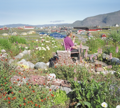
Saqqannguaq Road,
Narsaq, Greenland
FINN LARSEN
Changing Pathways
Expect changes and some surprises. These
taminants, the Arctic is not remote or isolated
are the main conclusions from a review of the
from the rest of the world. Human activities in
pathways by which contaminants are trans-
industrial and densely populated areas will
ported to, from, and within the Arctic and
continue to influence what was once thought
how these pathways might respond to shifts
to be a pristine environment.
in climate.
This chapter summarizes current knowledge
During the 1990s, wind and weather pat-
on contaminant pathways and how they relate
terns in the Arctic were quite different from
to climate change. It thereby provides further
the previous three decades. It is too early to
elaboration and discussion of some points
say whether this is part of a natural, recurring
raised in the chapters Persistent Organic Pollu-
change in climate regimes or the result of
tants, Heavy Metals, and Radioactivity, espe-
global warming. Nevertheless, the conditions
cially looking at time trends and future per-
provide some important indications about
spectives. The chapter touches on the effects of
how pathways can change and potentially
long-term climate change in the Arctic. This
alter the load of contaminants to different
topic will be treated in more depth in the forth-
parts of the Arctic. Despite the uncertainty,
coming Arctic Climate Impact Assessment
one truth still stands. When it comes to con-
(ACIA), due in 2004.
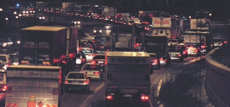
European Route E4,
Stockholm
POLFOTO / PELLE ERICHSSON
98
Changing Pathways
Climate change in the Arctic
Arctic Climate Impact Assessment
Climate change and variability, and, more
The Arctic is subject to natural climate cycles.
recently, notable increases in ultraviolet radi-
Some occur over time scales as short as a few
ation, have become important issues in the
years, while others may span decades, cen-
Arctic over the past few decades. Under the
turies, or even millennia. In addition to this
auspices of the Arctic Council, a program
natural variability, the Arctic will be affected
has been initiated to evaluate and synthesize
by global climate changes related to increases
knowledge about climate variability, climate
in greenhouse gases.
change, and increased ultraviolet radiation
The following is a short introduction to
and their consequences. This Arctic Climate
climate change and climate variability in the
Impact Assessment (ACIA) will also examine
Arctic.
possible future impacts on the environment
and its living resources, for example on hu-
man health, and on buildings, roads and
Global climate change
other infrastructure.
will warm the Arctic
Three major documents will be completed
by 2004. They are a peer-reviewed scientific
Human activities, such as the burning of fossil
report, a synthesis document summarizing
fuels, release greenhouse gases to the atmos-
results, and a policy document providing re-
phere. They affect the Earth's energy balance,
commendations for coping with and adapt-
which in turn has the potential to influence
ing to change. The writing of the first two
temperatures and weather patterns. Expert
documents is guided by an Assessment Steer-
opinion, as expressed by the Intergovernmen-
ing Committee with the lead authors, repre-
tal Panel on Climate Change, is that some
sentatives from the Arctic Monitoring and
changes are already apparent. This conclusion
Assessment Programme (AMAP), the Pro-
gram for the Conservation of Arctic Flora
is based on comparisons with past tempera-
and Fauna (CAFF), the International Arctic
ture records and indirect signs of climate var-
Science Committee (IASC), other interna-
iability during the past 1000 years. In the past
tional bodies, and persons representing the
century, the global mean air temperature has
Arctic indigenous peoples.
increased by 0.6 °C. Based on computer mod-
els of the effects of greenhouse gases on the
global climate, the Earth's air temperature
is expected to increase by an additional 1.4
annual mean air temperature may still in-
to 5.8°C over the next century. The range rep-
crease by 5°C near the pole and by 2-3°C
resents uncertainty about future emissions as
around the margins of the Arctic Ocean.
well as an uncertainty about their effects.
However, there are large regional variations,
Climate models show that the warming
even including cooling in some areas.
will be especially pronounced in the Arctic.
The greatest warming will probably occur
Excluding the more extreme predictions, the
in winter. By the end of the 21st century, some
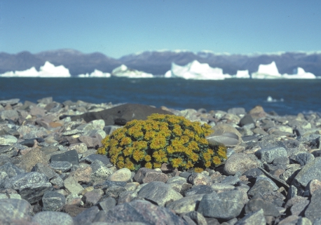
Large cluster of rose
root on stony shore.
Kangerterajiva, Green-
land.
POLAR PHOTOS / HENNING THING
Mean sea ice extent, million km2
Recent climate trends
99
12
follow from Arctic Oscillation
Changing Pathways
10
It is well known that climate can oscillate
Model projections of
8
between different climate regimes. El Nińo/
change in sea ice cover
La Nińa in the Pacific is one example outside
for the Arctic Ocean.
6
the Arctic. In the Arctic, these climate regimes
Annual mean sea ice
extent is shown for the
are characterized by a high or low Arctic
4
Northern Hemisphere as
Oscillation Index, which captures different
simulated by two different
2
regimes in atmospheric circulation (see box
climate models, which dif-
below). Wind and weather patterns affect ice
fer in how they treat mix-
0
1900
1950
drift and the distribution of water masses in
ing of the water mass.
2000
2050
2100
the Arctic, which in turn can change the extent
models predict that climate change caused by
of ice cover. Changes in air circulation can
greenhouse gases might produce an Arctic
thus influence the transport of contaminants
Ocean that is free of sea ice in the summer.
into and within the Arctic in several ways.
It is not clear to what extent global climate
Since the 1960s, there has been a change in
change has already affected the Arctic. How-
the overall pressure pattern in the Arctic. The
ever, current models predict changes that are
1990s in particular have been characterized by
consistent with observations made during the
lower than average atmospheric pressure over
1990s.
the pole. Expressed in a different way, a low
Winter
Winter Arctic Oscillation Index
0
+
4
0
1960
1970
1980
1990
2000
2
The Arctic Oscil-
lation Index since
1960 and the
North Atlantic
Oscillation Index
since 1900. The
Summer
maps represent a
combination of the
Summer Arctic Oscillation Index
Arctic Oscillation
0
+
Index and atmos-
1
pheric pressure
fields during win-
1
ter and summer.
2
1
1960
1970
1980
1990
2000
North Atlantic
+
Oscillation Index
1900
1920
1940
1960
1970
1980
1990
2000
The Arctic Oscillation and the North Atlantic Oscillation
A leading component of variation in the Arctic's climate is governed by the Arctic Oscillation, which captures different
regimes in atmospheric circulation in the northern hemisphere. Atmospheric circulation patterns can be described by differ-
ences in sea-level air pressure, or the barometer reading in layman's terms. The Arctic Oscillation Index is a measure of sea
surface air pressure patterns. Specifically, it captures winter pressure anomalies north of 20°North.
Strongly correlated with the Arctic Oscillation is the North Atlantic Oscillation, which is a measure of the surface air
pressure difference between the Icelandic Low and the Azores High. This index is an indication of the main wind patterns
over the North Atlantic.
100
Positive Arctic Oscillation Index
Negative Arctic Oscillation Index
(cyclonic)
(anticyclonic)
Changing Pathways
Aleutian Low
Winter
1015
1015
L
L
1015
1015
1015
1025
H
H
L
1005
L
1015
H
Icelandic Low
Siberian High
Positive Arctic Oscillation Index
Negative Arctic Oscillation Index
(cyclonic)
(anticyclonic)
Beaufort High
H
Summer
H
1018
1018
1014
1014
1010
1010
1014
1014
L
Atmospheric pressure
L
L
fields and wind patterns
1018
1010
1014
in winter and summer
1018
1006
with the Arctic Oscilla-
tion Index strongly posi-
tive (left) or strongly
H
H
negative (right).
Arctic Oscillation Index had been replaced by
ing the relative distribution of contaminants
a high Arctic Oscillation Index. The cause for
between the air, land, and ocean. Changes in
this shift is not completely understood. It could
wind patterns, precipitation, or temperature
be the result of natural climate cycles, where
can thus change the routes of entry of conta-
short- and long-term patterns have coincided
minants into the Arctic and the locations at
to produce a very high index in the 1990s.
which contaminants are deposited to surfaces
It could also be a sign of the Arctic responding
or re-emitted to the air.
to global climate change. Regardless of which
explanation turns out to be correct, the
Wind patterns govern pollution transport
changes observed in the early 1990s provide
an example of how the Arctic might respond
The Arctic is characterized by relatively pre-
to global warming, including examples of how
dictable patterns of sea-level air pressure.
climate change may alter the transport of con-
Every winter, high-pressure areas form over
taminants.
the continents, while low pressure cells domi-
nate the northern Pacific (the Aleutian Low)
and the northern Atlantic (the Icelandic Low).
Winds, precipitation
These low- and high-pressure areas pro-
and temperature
duce wind patterns that pump airborne pollu-
tants into the Arctic. The Icelandic Low pro-
The atmosphere provides an important path-
duces westerly winds over the eastern North
way for contaminant transport. Winds carry
Atlantic and southerly winds over the Nor-
contaminants from source regions, while pre-
wegian Sea, which can carry pollution rapidly
cipitation promotes deposition to the land and
from eastern North America and Europe into
the sea. Temperature plays a role in determin-
the High Arctic. Similarly, the Aleutian Low
tends to steer air from Southeast Asia into the
101
Bering Sea, Alaska, and the Yukon Territory.
Changing Pathways
Here, however, the mountains along the west
coast of North America obstruct the airflow,
while intensive precipitation on their western
flanks provides a mechanism to deposit conta-
minants to the surface.
In summer, the continental high-pressure
cells disappear and the oceanic low-pressure
cells are less intense. The result is much
weaker transportation of air and pollutants
into the Arctic from southern areas during
summer.
With a high Arctic Oscillation Index, as in
Difference in winter pre-
the 1990s, the Icelandic low deepens. More-
cipitation between low
over, it extends farther into the Arctic, across
and high North Atlantic
the Barents Sea and into the Kara and Laptev
Oscillation Index.
Seas north of Russia. This increases wind
transport eastward across the North Atlantic,
1.5
1.2 0.9
0.6
0
0.3
0.6
0.9
1.2 mm/ day
across western and central Europe, and into
Difference in winter precipitation
the Norwegian Sea. Also, deep storms with
strong winds become more frequent and ex-
used in many Russian and Eastern European
tend farther into the Arctic.
cars, rains out in the Nordic Seas and in the
The result of this shift in winter wind pat-
southern portion of the Eurasian Basin. Ocean
terns is that the Arctic becomes more strongly
transport is much slower than air transport
connected to industrial regions of North Amer-
and the pollution signal to various parts of the
ica and Europe. The storms also carry rain or
Arctic can thus be delayed.
snow, which can wash contaminants from the
The changes in winds and temperature that
air and deposit them on the ground, on ice, or
are associated with shifts in Arctic Oscillation
in the water.
are likely to affect precipitation. The network
The wind patterns in the Pacific appear to
to monitor changes is sparse, however, and it
change very little in a shift from a low to a
is thus difficult to assess trends. Over a longer
high Arctic Oscillation Index.
time span, the past 40 years, there are indica-
Changes in wind patterns will affect all air-
tions that precipitation has increased over Can-
borne contaminants. For example, spraying of
ada's North by about 20 percent. More mois-
pesticides in eastern North America and Eu-
ture is probably also moving into the Barents,
rope is more likely to show up as peaks in
Kara, and Laptev Seas, carried by the strong
Arctic air measurements during a high Arctic
southerly winds in the Norwegian Sea during
Oscillation Index. Similarly, re-emissions of
autumn and winter. Models for long-term cli-
previously deposited organic pollutants in the
mate change predict that the Arctic will be-
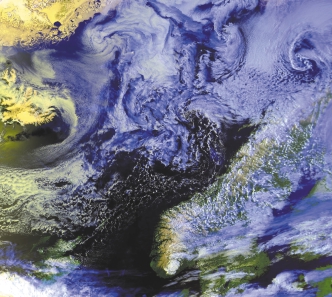
Storm over the Norwe-
soil and water of North America and Europe
come a wetter place, and a greater fraction of
gian Sea. Satellite image.
will enter these same pathways and thus be
transported more readily to the north. How-
ever, as we will see below, increased transport
by air can be offset by other factors.
Precipitation transfers pollutants
from the air to slower ocean currents
Air transport of particle-associated metals
such as lead, cadmium, and zinc will be af-
fected by changing wind patterns. However,
these pollutants are scavenged inefficiently
within the Arctic and thus tend to stay in the
air rather than deposit to the surface. The
actual load to land and sea surfaces in the
Arctic depends strongly on the amount and
kind of precipitation. Changes in snow and
rain patterns thus have a much greater poten-
tial to alter loading than does a change in
wind patterns.
Particulate metals wash out in high precipi-
tation areas. If this occurs over the sea, metals
can then be carried by ocean currents. For ex-
ample, lead from leaded gasoline, which is still
KONGSBERG SATELLITE SERVICES / NOAA
the atmospheric particles that enter the Arctic
extent dissolve in water, such as HCHs and
102
are thus likely to deposit there.
toxaphene. High precipitation in the Nordic
Changing Pathways
Snow and fog are far more efficient than
Seas and southern Eurasian Basin would thus
rain in removing some contaminants from the
increase the role of ocean currents and ice as
air and depositing them to the surface. For met-
pathways. In the Bering Sea, rainout has selec-
als, both a change in the amount of precipita-
tively removed beta-HCH from the air, and
tion or in the relative amounts of rain and snow
switched the mode of delivery to the Arctic
can thus have a large impact on transport.
Ocean from transport by winds to transport
In 1991, the Canadian air monitoring sta-
by ocean currents. Beta-HCH, a component
tion at Alert recorded a marked dip in aerosol
of the pesticide technical HCH, is especially
metal concentrations. It was noted that this
likely to move from air to seawater.
decrease coincided with the economic collapse
that followed the fall of the former Soviet
Most of the Arctic has become warmer
Union, which significantly reduced emissions
of some heavy metals in Russia. However, the
Parts of the Arctic have become warmer in the
air concentrations could also have been af-
past 40 years. In spring, surface air tempera-
fected by the shift toward a high Arctic Oscil-
tures in almost the entire High Arctic show a
lation Index that occurred at this time. It is dif-
significant warming. In the Eurasian part of
ficult to determine the relative importance of
the Arctic Ocean, there is a trend toward a
the two explanations without data that both
longer period of the year when the sea ice is
cover a wide range of sites and span several
melting. As an Arctic average, temperatures
climate change cycles. Nevertheless, the Alert
over land have increased by up to 2°C per
example illustrates that caution must be used
decade during the winter and spring. However,
in assigning causes for contaminants trends in
there are significant regional variations. For ex-
relatively short time series.
ample, on a yearly average basis, the western
Scavenging by rain and snow can also be
Greenland-Baffin Bay area has been cooling.
important for particle-associated POPs, such
Changes in air temperature can have a di-
as some PCBs, and for POPs that to some
rect physical effect on the transport of some
contaminants. This is true for substances
Temperature change,
whose volatility, solubility, and adsorption to
1961-1990,
solids are sensitive to temperature, which is the
°C per decade
case for most POPs. The previous AMAP
0.6 - 0.8
assessment described how volatile contami-
0.5 - 0.6
nants can reach the Arctic from their source
0.4 - 0.5
regions in the south by a series of `hops'.
Higher temperatures in the Arctic would lead
0.2 - 0.4
North Pole
to an increased potential for atmospheric
0.1 - 0.2
transport. Previously deposited organic pollu-
0.2- 0.1
tants would also be volatilized once again and
move back into the atmosphere. On the other
0.3- 0.2
hand, if the temperature difference between
0.4- 0.3
the pole and equator decreases, as predicted
0.5- 0.4
by models, the global thermodynamic contrast
that favors the Arctic as a final reservoir would
weaken. Higher temperatures could also speed
up some of the chemical reactions that remove
pollutants from the atmosphere. Increases in
Temperature anomaly, °C
55-85°N
ultraviolet radiation, which are connected to
Temperature trends for
1.0
ozone depletion in the Arctic, also promote
the Arctic showing the
annual surface tempera-
chemical reactions that destroy or change the
0.5
ture trends over the
form of contaminants.
Average 1951-1980
Northern Hemisphere
0
Even more important than the effects on air
expressed as rates of
0.5
chemistry might be that higher temperatures
change for the period
will lead to more efficient degradation of con-
1961-90 (map), tempera-
1.0
ture anomalies (55-85° N)
1900
1920
1940
1960
1980
taminants by aquatic microorganisms. For
for 1900-1995 evaluated
alpha-HCH, a simple calculation shows that a
against the average for
Temperature change per decade, °C
significant increase in temperature in the upper
1951-1980, and (lower
0.6
water layers of the Arctic Ocean could sub-
panel) the trend by month
Central Arctic Ocean
stantially reduce the environmental half-life of
in surface air tempera-
0.4
ture of the central Arctic
this substance. One model has tried to predict
Ocean for the period
0.2
how an increase in temperature would change
1979-1995 showing the
the health risk from hexachlorobenzene (HCB)
recent warming to be
0
to people in a temperate region. HCB poses a
mainly a winter-spring
phenomenon.
health risk partly because it biomagnifies in
0.2
J
F
M
A
M
J
J
A
S
O
N
D
marine food webs and can reach people from
traditional foods. The model implied a reduced
lakes farther south. Specifically, the water col-
103
exposure with increasing temperatures. The rea-
umn will mix earlier, increasing the likelihood
Changing Pathways
son is that higher temperatures would enhance
that contaminants will be retained in the lake.
degradation and also force this pollutant from
Moreover, the warmer water, along with wind
water into the air, reducing the water concen-
mixing and more organic matter from the sur-
tration and, therefore, reducing the amount of
rounding land, may influence primary produc-
HCB entering the bottom of the food web.
tion. A change in the amount or timing of pri-
mary production may increase the opportunity
for contaminants to enter the food web directly.
Changing water flows in rivers
However, it could also lead to more sedimenta-
Changes in temperature and precipitation will
tion, which, at least temporarily, removes con-
affect runoff and flow in Arctic rivers. So far,
taminants to the bottom sediments.
changes in flow seem to be within normal year-
to-year variability. With long-term climate
Permafrost changes may increase
changes, models suggest that the flow in the
mercury cycling and natural radioactivity
Yenisey, Lena, and Mackenzie Rivers is likely
to increase. In other rivers, such as the Ob, it
In the Arctic, ice is a more or less permanent
may decrease. For smaller rivers at high lati-
feature on land. The soil is typically gripped in
tudes, the seasonal patterns of river flow are
permafrost, and only the relatively thin active
likely to change. It is projected that earlier
layer on top thaws in the summer. This layer,
snowmelt in spring would change the timing,
which supports all biological processes and
amplitude, and duration of spring flow.
any vegetation, can be limited to the top meter
There are also some changes in where river
or less. In the 1990s, permafrost degradation
water goes once it has entered the ocean. This
occurred in some parts of Alaska and Russia,
is discussed in the section New pathways in
but not in northeastern Canada. This matches
Arctic Ocean surface waters on page 105.
the distribution of air temperature trends
observed and predicted by climate models.
Permafrost melting will lead to more nutri-
Lakes, land, and glaciers
ents and sediments reaching lakes and rivers.
The flow of organically bound carbon and
Ice can act as a physical barrier for contami-
mercury may also increase. Episodic, large-
nants and also, at times, as a reservoir. What
scale releases of organically bound mercury
happens when higher temperatures melt ice in
may become a dominant feature accompany-
lakes, in the ground, and in glaciers?
ing permafrost degradation. Clearly, Arctic
Lakes are sensitive to changes
Arctic lakes are sensitive to climate change,
as temperatures directly affect the timing of
freeze up in the fall and ice melt in spring.
This, in turn, affects the flow of water to,
within, and from the lake. There are no studies
that show effects of changes in the Arctic Os-
cillation Index on Arctic lakes. In North Amer-
ica, long-term change has been observed, how-
ever. Over the past 100 years, there has been a
delay of several days in freeze-up, while the
spring break-up now comes almost a week ear-
lier than it did a century ago. Changes in water
flow through lakes can have a large impact on
MAGNUS ELANDER
the transport of contaminants. Currently, Arc-
tic lakes appear to retain only a small fraction
lakes would be vulnerable, but increased input
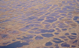
Aerial view of polygon
of the contaminants they receive. The peak in
of carbon is also projected for Arctic seas, sug-
tundra, Lena Delta,
runoff from the snowmelt in their catchment
gesting an increased load of mercury, which
Russia.
areas comes before the ice on the lake has
follows the carbon, in the marine environment.
melted or before the water in the lake has
Hudson Bay may be especially vulnerable due
begun mixing from top to bottom, as it does
to its large drainage basin and because perma-
when the lake warms up in summer. The run-
frost melting is likely in the area. Mercury con-
off, which contains recently deposited contam-
centrations in snow have increased in this area,
inants, therefore traverses the lake just under
as have mercury fluxes to sediment.
the ice or above most of the water column,
Along the coasts, sea-level rise will promote
flowing out as quickly as it flows in.
erosion, which could disturb contaminated
With the reduced ice cover and loss of per-
sites. It may also damage structures such as
mafrost that is expected with climate change,
pipelines, thus releasing potentially contami-
Arctic lakes will probably become more like
nating substances to the environment.
shrinking since the 1960s. In the Canadian
Archipelago, the glacial melt was exceptionally
strong in the 1990s, corresponding to the high
Arctic Oscillation Index. In the European Arc-
tic, the trend is not as clear. Scandinavian glac-
iers have grown during the 1990s, whereas
most Svalbard glaciers continue to shrink at
the same rate as they did throughout the 1900s.
Russian glaciers may be retreating, but this is
difficult to establish because of limited data.
Measurements from the Agassiz Ice Cap in
Canada give a hint of the size of glaciers as a
potential source for contaminants. For DDT,
glacial melt may provide an important climate-
modulated source. For HCHs and PCBs, this
source is small compared with the reservoir in
the Arctic Ocean.
POLAR PHOTOS / HENNING THING
Ocean transport
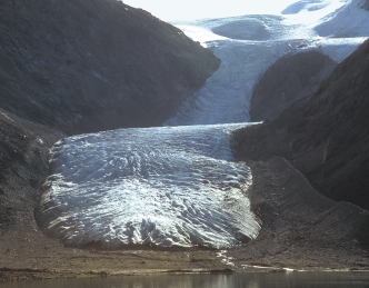
Glacier at Kangerlus-
Change in permafrost also has an implica-
The Arctic Ocean is divided into distinct lay-
suatsiaq, West Green-
tion for radon that diffuses out of the ground.
ers. Below 800 meters is Arctic deep water,
land. The light grey
This radionuclide is not generally related to
with a very long residence time. From 200 to
zones at each side of the
anthropogenic activities but comes from soils
about 800 meters is the Atlantic Layer. At the
glacier show the former
extent.
and bedrock. Radon is trapped in frozen
very top is the Arctic surface water, which is
ground in the Arctic, but with warmer temper-
the most important for contaminant transport
atures, more radon will diffuse out of soils,
within the Arctic Basin. Between the surface
increasing the dose of this element and its
water and the Atlantic layer is the halocline,
decay products to people.
a transition zone of increasing salinity. The sig-
nificance of ocean transport for contaminants
to, from, and within the Arctic has been in-
Glaciers could become sources of DDT
creasingly recognized during the past few
Glaciers have accumulated snow and ice over
years. Currents are sluggish compared with
millennia. They also act as reservoirs for some
winds, and oceans therefore become important
airborne contaminants. When the glaciers
later in a contaminant's history. However, the
melt, these contaminants can be re-emitted to
ocean may have a much larger capacity to
the air or be released in the meltwater. In the
carry contaminants than the air, allowing cur-
Arctic, North American glaciers have been
rents eventually to catch up with and surpass
Ice
Normal placement of the Atlantic-Pacific front Polar mixed layer
Atlantic-Pacific front
Pacific halocline
during high Arctic Oscillation Index, early 1990s
Atlantic halocline
Bering Strait
Fram Strait
Depth, m
75°N
80°N
85°N
90°N
85°N
80°N
0
ca. 10 years
Bering
200
Pacific water
ca. 10 years
Strait
400
Atlantic water
ca. 25 years
600
ca. 30 years
Atlantic layer
800
1000
Fram
Strait
Arctic deep water
Norwegian Sea
and Greenland Sea
ca. 75 years
deep water
The stratification of
2000
the Arctic Ocean.
Canada
Makorov
showing the polar
Basin
Basin
mixed layer, the
Alpha
Pacific and Atlantic
Ridge
domains of influence
3000
ca. 300 years
Amundsen
Nansen
and the haloclines.
Basin
Basin
The red lines show
the normal placement
ca. 290 years
Nansen
and the displacement
Lomo-
Gakkel
nosov
of the Atlantic Pacific
Ridge
Ridge
front during the high
4000
Arctic Oscillation
Bold figures denote residence times
Index of the early
1990s.
1979
1990-1994
105
Freshwater runoff distribution
Russia
Salinity
Low
Greenland
Alaska
High
620
430
85
525
Changes in the distribu-
tion of freshwater runoff
600+
in the Arctic Ocean be-
600+
Atlantic-Pacific
2000
tween low Arctic Oscil-
Front
Atlantic-Pacific
Front
lation Index, 1979, and
200
high Arctic Oscillation
200
?
Index, 1990-94 (upper
maps), and changes in
Pre 1990
Post 1990
330
330
the amounts of river in-
Low Arctic Oscillation Index
High Arctic Oscillation Index
River inflow, km3/year
River inflow, km3/year
flow to the Arctic Ocean
under same conditions.
atmospheric transport in importance. Some of
reduction in stratification in the Eurasian
the ocean pathways have already exhibited
Basin and increased stratification in the Can-
changes clearly related to the Arctic Oscillation.
adian Basin.
The diversion of the Russian river outflow
affects the transport of persistent organic pol-
New pathways
lutants both from the rivers and within the Arc-
in the Arctic Ocean surface waters
tic Ocean. Specifically, instead of entering the
Surface ocean water pathways follow two
Transpolar Drift to exit the Arctic Ocean with-
basic trajectories: the Transpolar Drift that
in about two years, the pollutants would enter
crosses the Eurasian Basin and exits through
the Canadian Basin, which has a ten-year resi-
Fram Strait, and the circulating Beaufort
dence time. Pollutants would thus stay in the
Gyre on the North American side of the
Arctic Ocean much longer, especially increas-
Arctic Ocean (see figure on page 3). With a
ing the load in the Canadian Basin. Further-
high Arctic Oscillation Index, water in the
more, once in the Canadian Basin, pollutants
Transpolar Drift moves closer to North
from Russian rivers might then exit via the
America, while the Beaufort Gyre retreats
Canadian Archipelago instead of via the west
into the Canadian Basin.
side of Fram Strait. The increased residence
More important than changes in trajectories
time would lead to increased sedimentation,
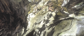
Driftwood from Siberia
found at Fleming Fjord,
are the effects on the halocline. This is a transi-
making it likely that more sediment-bound
north of Ittoqqortoor-
tion zone of increasing salinity, which serves as
contaminants would remain in the Arctic.
miit, East Greenland.
a barrier for transfer of heat and contaminants
from Arctic surface water to the Atlantic water
below. In the 1990s, the halocline in the Eur-
asian Basin weakened. The most likely reason
was that changes in wind patterns forced
freshwater from the Russian rivers emptying
into the Laptev and Kara Seas eastward, di-
verting their flow toward the East Siberian
Shelf. The freshwater input to the Arctic Ocean
is important for the development of stratifica-
tion in the water column. A consequence of
this diversion, therefore, would have been a
POLAR PHOTOS / HENNING THING
marine environment. In the past few decades,
106
High North Atlantic Oscillation Index
the North Atlantic Oscillation Index has in-
Changing Pathways
creased, causing changes in distribution of
water masses in the Nordic Seas. This has
brought contaminants from the reprocessing
plants closer to the Norwegian coast and into
the Barents Sea.
Traditionally, the Arctic Ocean has been
thought of as a quiet, steady-state system char-
acterized by several relatively stable layers.
During the 1990s, there were some spectacular
changes. The front between Atlantic and Pa-
cific water was forced closer toward North
America, which increased the Atlantic's area of
influence in surface water by some 20 percent.
Water in the Atlantic layer is both warmer and
Low North Atlantic Oscillation Index
saltier than the Pacific water that it displaced.
The declining role of Pacific water in the
Barents
Arctic Ocean has implications for cadmium,
Sea
a toxic metal that biomagnifies in the marine
Greenland
food web. In the ocean, the distribution of this
Sea
metal is largely controlled by natural biogeo-
Norwegian
Sea
chemical cycles, with the Pacific having higher
Iceland
Sea
natural concentrations than the Atlantic. Be-
cause the Pacific inflow through the Bering
Irminger
Strait is a dominant source to the surface
Main features of ocean
Sea
Labrador
waters of the Arctic, reduced Bering inflow
circulation in the North
Sea
since the 1940s has probably led to reduction
Atlantic and the Nordic
Seas during high and low
in cadmium input. Furthermore, the encroach-
North Atlantic Oscilla-
Atlantic water
Arctic water
ment of Atlantic water during the recent high
tion Index.
Arctic Oscillation Index will have reduced the
The Atlantic's increased role leads to
domain of Pacific water that is relatively en-
declines in cadmium
riched with cadmium within the Arctic. Changes
in upwelling or mixing are also likely to affect
For the Atlantic Layer, the Arctic Oscillation
the entry of cadmium into surface water from
influences the flow of water into and out of the
deeper layers.
Arctic Ocean. Communication with the Pacific
is through Bering Strait, while communication
An exceptionally strong
with the Atlantic is through Fram Strait and
shift to high Arctic and
Sea ice
through the Norwegian and Barents Sea. Im-
North Atlantic Oscilla-
tion Indices in about
portant contaminants in the Atlantic inflow
One of the prominent features of the Arctic
1989 increased the influ-
include radionuclides from European repro-
Ocean is its ice cover. Changes in ice cover
ence of Atlantic water
cessing plants, and any change in the flow of
have already occurred and the effects of this
(red) in the Arctic basin.
Atlantic water may thus affect concentrations
on persistent organic pollutants and mercury
The Atlantic layer cur-
rents are relatively fast
and distribution of radionuclides in the Arctic
may become increasingly important.
and move water at a rate
of 300-1600 kilometers
Low Arctic Oscillation Index
High Arctic Oscillation Index
per year along the mar-
gins of the basin.
Alaska
Temperature
Warm
Russia
Cold
Greenland
Winter maximum
Summer minimum
107
;;;;;;;;;;;;;;;;;;;;;;;;;;
Changing Pathways
;;;;;;;;;;;;;;;;;;;;;;;;;;
;;;;;;;;;;;;;;;;;;;;;;;;;;
;;;;;;;;;;;;;;;;;;;;;;;;;;
;;;;;;;;;;;;;;;;;;;;;;;;;;
;;;;;;;;;;;;;;;;;;;;;;;;;;
;;;;;;;;;;;;;;;;;;;;;;;;;;
;;;;;;;;;;;;;;;;;;;;;;;;;;
;;;;;;;;;;;;;;;;;;;;;;;;;;
;;;;;;;;;;;;;;;;;;;;;;;;;;
;;;;;;;;;;;;;;;;;;;;;;;;;;
Total ice cover
;;;;;;;;;;;;;;;;;;;;;;;;;;
;;;;;;;;;;;;;;;;;;;;;;;;;;
;;;;;;;;;;;;;;;;;;;;;;;;;;
;;;
Partial ice cover
;;;;;;;;;;;;;;;;;;;;;;;;;;
;;;
;;;;;;;;;;;;;;;;;;;;;;;;;;
;;;
Open water
;;;;;;;;;;;;;;;;;;;;;;;;;;
;;;;;;;;;;;;;;;;;;;;;;;;;;
;;;;;;;;;;;;;;;;;;;;;;;;;;
;;;;;;;;;;;;;;;;;;;;;;;;;;
;;;;;;;;;;;;;;;;;;;;;;;;;;
Winter maximum and
;;;;;;;;;;;;;;;;;;;;;;;;;;
;;;;;;;;;;;;;;;;;;;;;;;;;;
summer minimum Arctic
;;;;;;;;;;;;;;;;;;;;;;;;;;
sea ice cover as derived
;;;;;;;;;;;;;;;;;;;;;;;;;;
from satellite imagery.
than multi-year ice because it is thinner and
Less ice cover
saltier. In the East Siberian and Beaufort Seas,
During the 1990s, the scientific community
there were unusually large areas of open water
recognized with some alarm that Arctic sea ice
in late summer at various times during the
had retreated over the past three decades. The
1990s. It appears that the marginal seas are
changes included a reduction in the area cov-
becoming only seasonally covered with ice,
ered by sea ice, an increase in the length of the
and that the extent of the permanent ice pack
ice melt season, and a loss of multi-year ice.
is decreasing.
The rate of loss has been difficult to estimate
The loss of sea ice is consistent with what
but is approximately 3 percent per decade.
can be expected under a high Arctic Oscil-
Most of the ice has been clearing during
lation Index. Several factors are probably
summer over the shelves of the Eastern Arctic,
involved including more heat being trans-
north of Russia. Multi-year ice has decreased
ported to the pole by southerly winds. Even
even more rapidly and been partly replaced by
more important might be that winds cause
first-year ice. First-year ice melts more easily
changes in the distribution of ice. Ice-thickness
measurements made from submarines indicate
Sea ice extent, million km2
that the multi-year ice in the Central Arctic
8.0
Ocean has been getting thinner. Most of the
Monthly averages
7.0
information has been gathered in the interior
of the Arctic Ocean, and the decrease might
6.0
be, at least in part, the product of a shift in the
5.0
distribution of multi-year ice toward North
4.0
America.
Sudden but temporary changes in ice cover
1.0
Monthly deviations
have occurred earlier in Arctic history. Over a
0.5
century ago, the whaling fleet experienced a
0
dramatic decrease in ice cover in the North
American Arctic. In the Barents Sea, about 15
0.5
percent of sea ice cover was lost around 1920.
1.0
1980
1985
1990
1995
Increased exchange of POPs
Sea ice extent,
change per decade, %
between sea and air
0.5
Some persistent organic pollutants have accu-
0
mulated in the Arctic Ocean surface waters.
0.5
The low temperatures of the Arctic, which
1.0
decreases their volatility in air and increases
1.5
their tendency to dissolve in water, acts as a
2.0
driving force in moving them from the air to
The change in Arctic
Ocean sea ice extent
2.5
the water. This pathway is especially important
from 1979 to 1995
for compounds that prefer cold water, alpha-
showing the ice loss to
3.0
HCH being a prime example. Once these pollu-
be predominantly a late
3.5
tants are in the water, they can become trapped
wintersummer phenom-
4.0
enon.
J
F
M
A
M
J
J
A
S
O
N
D
under the ice and retained in the water masses,
Month
some of which have long residence times.
108
Low Arctic Oscillation Index
Russia
High Arctic Oscillation Index
Changing Pathways
Transpolar Drift
Transpolar Drift
Beaufort Gyre
Beaufort Gyre
Ice drift patterns for
years with low and high
Canada
Greenland
Arctic Oscillation Index.
For alpha-HCH, discontinued use of the
deposition would decrease, and at the same
pesticide technical HCH has led to a drastic
time more mercury could escape back to the
reduction in air concentrations. As a conse-
atmosphere after being deposited. The end
quence, the ice-covered areas of the Arctic
result would be less accumulation of mercury
Ocean became oversaturated relative to atmos-
in marine and aquatic environments. It is
pheric levels. If the ice cover disappears, these
harder to predict whether levels in biota
areas will become a source to the atmosphere.
would also change. Mercury biomagnifies
Other contaminants, such as PCBs and toxa-
and its levels depend on the structure of the
phene, are still loading into the Arctic Ocean
food web. Changes in the food web structure
from the air. The same loss of ice cover could
could, therefore, be much more important
thus lead to increased loading of these two
than changes in physical pathways. Mercury
contaminants into Arctic surface water.
levels may also be affected by changes in per-
mafrost, and increase with an increased flux
of organic carbon to both freshwater and
Ice changes will affect
marine environment. In summary, the com-
mercury deposition in the Arctic
plexity of mercury pathways combined with
As described in the chapter Heavy Metals,
obvious sensitivities to climate change should
mercury deposition in the Arctic increases dra-
alert us to the possibility of surprises in the
matically at polar sunrise due to an extraordi-
future.
nary set of circumstances. The phenomenon is
called mercury depletion. Although the mech-
Shifting routes from drifting sea ice
anisms behind mercury depletion are not yet
fully understood, results of investigations to
The general patterns of ice drift have been rec-
date indicate that gaseous mercury in the air
ognized since the beginning of the 1900s, and
reacts with bromine compounds to form par-
follow the same trajectories as ocean surface
ticulate and reactive mercury. The bromine
water in the Transpolar Drift and the Beaufort
compounds are formed when bromine, emitted
Gyre. Only recently have these ice trajectories
from seawater and sea salts, reacts with ozone
been mapped in detail. The new data suggest
in the presence of ultraviolet light (hence the
that there are two characteristic modes of ice
connection to the return of the sun). The reac-
motion, one during a low Arctic Oscillation
tive mercury that is produced is efficiently re-
Index and one during a high index. During a
moved from the atmosphere and some of it
low index, which prevailed from the 1960s to
remains in the snow. Some will eventually end
the 1980s, the Transpolar Drift moves ice di-
up in meltwater and may thus enter aquatic
rectly from the Laptev Sea across the Eurasian
ecosystems. The sensitivity of the Arctic to
Basin and into the Greenland Sea. By contrast,
mercury probably lies in the fact that meltwa-
during a high index, the prevailing situation
ter and runoff can drain into surfaces below
for much of the 1990s, this ice transport route
the ice, where ice cover blocks the re-emission
is diverted or splits. Some goes to the Green-
of mercury to the air.
land Sea and some moves across the Lomono-
Change in sea ice cover can affect this
sov Ridge and into the Canadian Basin. At the
unique deposition mechanism if the availabil-
same time, the Beaufort Gyre shrinks back into
ity of bromine is altered. Initially, it is likely
the Beaufort Sea and becomes disconnected
that climate change will contribute to increas-
from the rest of the Arctic Ocean. This means
ing the amount of first-year ice around the
that it exports less ice to the East Siberian Sea
polar margins, leading to saltier ice and snow.
and only imports a little ice from north of the
It could thus enhance the emission of bromine
Canadian Archipelago.
and possibly extend the area of mercury deple-
The changes in ice-drift patterns have impli-
tion events.
cations for the transport of sediment and any
With further climate change, parts of the
contaminants trapped in the ice. Specifically,
Arctic will become more temperate. Mercury
when ice moves away from the East Siberian
and Laptev Seas, new thin ice can form close
spawning grounds to their nursery areas.
109
to the coast, increasing the opportunity for
Atlantic cod and its main food item capelin
Changing Pathways
sediments to be trapped. Moreover, less ice
are likely to move northeastwards. Spring-
moves from the North American to the Eur-
spawning herring may return to the same
asian part of the Arctic Ocean.
migration route they followed in the mid-
1960s, when the water temperature around
Iceland was higher than today. Other more
Biological impacts
southerly species may become distributed
Climate change will have impacts on plants
and animals in the Arctic and thus on the bio-
logical pathways for contaminants. Although
Capelin
we can infer the types of changes that are
likely to occur, we cannot predict their scope
and timing. The following are examples of
Cod
processes that should be examined further.
N O R W E G I A N S E A
Changing plant cover
will affect deposition
Herring
Vegetation provides surfaces onto which air-
borne contaminants can deposit when air
Mackerel,
Mackerel
blue tuna
masses pass over the land. Forests, for exam-
ple, have a unique ability to take chemicals
North Sea
herring
from the air via foliage and thence to a long-
Possible changes in the
term reservoir in the soil.
distribution of fish spe-
cies if the seawater tem-
Warmer winters will promote growth of
Anchovy, sardine
perature increases 1-2 °C.
woody shrubs and stimulate a northward
migration of the treeline. So far, there is no
farther north toward and into the Arctic. This
evidence of large changes on the Arctic tundra.
will lead to the introduction of new species
However, if permafrost melts and the water
into the Arctic marine ecosystem. The conse-
table changes, such changes could occur much
quences are difficult to predict but may include
more rapidly in the Arctic than in other regions
changes in the food web and thus in the load
of the world.
of contaminants in biota. Another possibility
is changes in migratory routes and contami-
nants along the route.
Aquatic ecosystems
are sensitive to changes
Changes in sea ice
Not only temperature but also changes in light
can alter marine ecosystems
and the flow of nutrients will affect freshwater
ecosystems. For example, loss of permafrost
In marine ecosystems, many contaminants are
will increase inputs of nutrients from the sur-
biomagnified in food webs, particularly those
rounding soil. Spring algae blooms will prob-
with many trophic levels. Therefore, any
ably come earlier.
changes in food web structure can potentially
In the summer, increased water temperature
have a large impact on contaminant burdens in
will negatively affect fish species that are sensi-
top predators. The changes can be initiated at
tive to temperature or have temperature thresh-
the bottom of the food web, for example if
olds during their spawning. Each species has to
changes in light and nutrient cycles alter con-
be evaluated separately, but trout and grayling
ditions for phytoplankton and zooplankton.
are known to be sensitive. Increased winter
Food-web changes can also be initiated at the
temperatures will enhance microbial decompo-
top, by altering predation patterns, for exam-
sition. Insects, phytoplankton, and zooplank-
ple among bears and seals.
ton will also be affected, some positively and
The amount of sea ice influences both light
some adversely.
conditions and the distribution of nutrients in
Along the North American Arctic coast, the
the water. Change in stratification of the
loss of estuarine ice may displace cisco, which
water column is important in this respect and
might be replaced by anadromous fish from
a decrease in mixing of water layers has
the Pacific Ocean.
already been noted in the Greenland Sea and
For marine fish, it is well known that
in the Canadian Basin. The availability of
changes in climate or ocean currents can affect
nutrients influences the algae that are respons-
the distribution of commercially important
ible for primary production at the bottom of
stocks, such as Atlantic cod and herring. Water
the food web. This is true for the phytoplank-
temperatures are important, as are the distrib-
ton in the water column and also for the algae
ution of prey and predators and the currents
that grow on the bottom of the ice and sup-
that determine the movement of larvae from
port a unique ice-associated food web. Some
of the algal production falls to the bottom of
this bird species. The change in quantity of
110
the ocean, where it supports the benthic food
different zooplankton probably also decreased
Changing Pathways
web. The distribution of sea ice thus has a
food availability for fish, whales, seals, and
major impact on the distribution of organic
walrus, causing die-offs and long-distance
matter between the water column and the
displacements.
seabed.
Loss of sea ice would lead to Arctic shelf
The Beaufort and Chukchi Seas, crossed
seas looking more like temperate seas. The
during the drift of the SHEBA (Surface Heat
implications for food web structures are very
Budget of the Arctic Ocean) Project in 1997-
difficult to predict and we should be prepared
98, provide a dramatic example of a large-
for surprises. One such warning sign was the
scale bottom-up change in the marine food
massive blooms of jellyfish in the Bering Sea
web. Compared with a study 20 years earlier,
during the 1990s. Large-scale changes pro-
this new close look at life in the water revealed
duced by the Arctic Oscillation have the poten-
a marked decrease in large diatoms and large
tial to alter the balance between upwelling and
microfauna within the ice. The high Arctic
downwelling along the coast, through changes
Oscillation Index of the 1990s had diverted
in either the distribution of ice cover or in
river water into this area, causing a strong
average wind speed and direction. Shifts in the
stratification of the surface waters. The result
Arctic Oscillation thus have the capacity to
was a decrease in the supply of nutrients from
cause large-scale shifts in shelf ecosystems. In
below, and a species composition that was
regions that are important for commercial fish-
more typical of freshwater ecosystems. The
eries, such changes can have major impacts on
loss of large diatoms could potentially produce
the regional economy.
a shift toward smaller zooplankton grazers,
Sea ice is also a crucial habitat for many
perhaps then introducing an extra step at the
species at the top of the food web. Ringed
bottom of the food web.
seals need landfast ice for pupping, which in
turn influences the migration of polar bears
that feed on the ringed seals. A decrease in
suitable habitat for ringed seals to pup could
lead to declines in their populations, with the
possible consequence that polar bears could be
forced to find other food sources or starve.
Ringed seals feed on Arctic cod. If changes in
the ice alter the balance between seals and
polar bears, they would likely affect the Arctic
cod as well.
Walrus provide an excellent example to
challenge our predictive capability. Most wal-
rus feed on bottom-dwelling organisms and
are thus fairly low in the food web. Some wal-
rus, however, are known to eat seals, and their
higher position in the food web is reflected in
higher contaminant levels. Many walrus use
drifting ice for their haulouts because it pro-
vides good access to nearby feeding areas,
reducing the amount of energy required to
feed. If the summer ice edge retreats north of
the relatively shallow areas where walrus can
feed, as happened in the summer of 1998 in
the Chukchi Sea, the walrus may be forced
either to starve or to prey on seals. The latter
adaptation would place walrus much higher in
the food web.
Less sea ice could, however, benefit other
species. Eiders, which also feed on the ben-
M A G N U S E L A N D E R
thos, need open water in which they can dive.
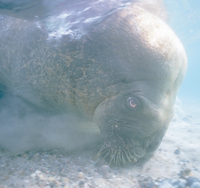
Walrus grazing on mussels.
The Bering Sea provides another recent
By benefiting some species and hindering oth-
Most walrus feed low in the
example of how bottom-up changes can per-
ers, the loss of sea ice is likely to cause major
food web, for example by
meate an entire ecosystem. In 1997-98, there
alterations in the marine food web. This is
grazing on mussels. How-
were massive blooms of small phytoplankton.
particularly true for changes caused in certain
ever, some individuals hunt
seals, thus receiving higher
Because they were smaller than the diatoms
key species. Arctic cod, for example, plays a
contaminant intakes. If cli-
that typically bloom in the Bering Sea, they
central role linking lower levels of the food
mate change were to cause
were grazed on by copepods instead of
web to seals, beluga, and many birds. Any
a shift in feeding habits, it
euphausiids. The short-tailed shearwater nor-
changes to Arctic cod abundance or distribu-
would thus have implica-
tions for contaminant lev-
mally feeds on the euphausiids, and the lack of
tion could propagate both up and down the
els in this species.
food may have contributed to a large die-off of
food web.
111
Changing Pathways
Tourists visiting the
North Pole on an ice-
breaker cruise take the
BRYAN & CHERRY ALEXANDER
Polar Plunge.
transport of airborne pollutants from eastern
Human activities will increase
North America and Eurasia. Another example
Climate change will inevitably bring changes to
is Atlantic water carrying more radionuclides
human activities in the Arctic, with subsequent
from European processing plants. Lead that
effects on contaminant loads and pathways.
has been deposited in the ocean to the west
For people, food habits have a great impact
of Europe would also follow this pathway.
on exposure to contaminants. Changes in
A third example is the longer residence time
hunting opportunities because of changed ani-
in the Arctic Ocean for contaminants that are
mal distribution and availability or changed
carried by ocean surface waters.
ability to travel over ice or land will thus have
Long-term climate changes are likely to
an impact. If a hunted animal is suddenly
affect pathways that are influenced by sea ice.
higher in the food web, its contaminant load
Such pathways will be important for many
could increase, thus increasing exposure even
persistent organic pollutants that partially
for people whose food habits remain the same.
dissolve in water, some of which are currently
A warmer Arctic with less sea ice will also
trapped under the ice. Mercury is likewise
encourage shipping, tourism, and oil exploita-
trapped under ice. For mercury, changes in sea
tion, all of which increase the risk for contami-
ice cover may also influence newly discovered
nation of new areas. More severe storms
physical pathways that enhance the deposition
would further increase risks connected to ship-
of mercury to surfaces.
ping and other offshore activities. The expan-
Changes in lake ice and permafrost will
sion of commercial fisheries from the Arctic
affect lake hydrology, potentially increasing
marginal seas into the Arctic Ocean would
the input of contaminants into freshwater
also likely affect food web structure and rela-
ecosystems and possibly releasing contami-
tive abundance of many species. Although the
nants that have accumulated in soil or have
net effects of changes in human activities and
been improperly disposed of in earlier times.
behavior in the Arctic are impossible to predict
Many contaminants pose a problem in the
with confidence, changes are certain to occur.
Arctic because they biomagnify in food webs.
They, in turn, will affect sources, pathways,
Changes in food web structure, therefore,
and eventual fate of contaminants in the Arc-
have a great potential to alter contaminant
tic, including human exposure.
levels in top predators. However, the com-
plexity of ecosystems and our incomplete
understanding of the dependence of many
Summary
species on habitats like sea ice make it espe-
cially difficult to predict change, and one
Long term-climate change and natural climate
should expect surprises.
cycles affect the transport of contaminants to
A final conclusion is that the load of per-
and within the Arctic. The 1990s provided an
sistent organic pollutants, heavy metals, and
example of how widespread change can rapidly
radionuclides in the Arctic is dependent on
pervade much of the Arctic including winds,
many factors that operate after the contami-
weather patterns, ocean currents, and sea ice.
nant has been released from its source. In the
It is, however, difficult to predict whether long-
long run, anthropogenic emissions that affect
term climate change will lead to a generally
the climate may become as important as the
decreased or increased contaminant load.
emissions of the contaminants themselves in
Some pathway changes clearly lead to more
determining the extent to which these con-
efficient transport, one example being increased
taminants reach and affect the Arctic.